anytime algorithms for learning anytime classifiers saher ... - Technion

Technion - Computer Science Department - Ph.D. Thesis PHD-2008-12 - 2008
Test costs
a1
a2
a3
a4
a5
a6
10
10
10
10
10
10
MC costs
FP
FN
100
100
r = 1
T1 T2
5
95
+
-
EE = 7.3
a3
- +
a1
a5
- +
95 + 5 + 95 +
5 - 95 - 5 -
EE = 7.3 EE = 7.3 EE = 7.3
mcost (T1) = 7.3*4*100$ / 400 = 7.3$
tcost (T1) = 20$
total(T1) = 27.3$
0
50
+
-
EE = 1.4
a4
- +
a2
a6
- +
100 + 0 + 100 +
50 - 50 - 50 -
EE = 54.1 EE = 1.4 EE = 54.1
mcost (T2) = (1.4*2 + 54.1*2) * 100$ / 400 = 27.7$
tcost (T2) = 20$
total (T2) = 47.7$
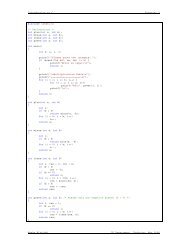
Figure 4.4: Evaluation of tree samples in ACT. The leftmost column defines the
costs: 6 attributes with identical cost and uniform error penalties. T1 was sampled
for a1 and T2 for a2. EE stands for the expected error. Because the total cost of
T1 is lower, ACT would prefer to split on a1.
Test costs
a1
a2
a3
a4
a5
a6
40
10
10
10
10
10
MC costs
FP
FN
100
100
r = 1
T1 T2
a3
- +
a1
5 + 95 + 5 + 95 +
95 - 5 - 95 - 5 -
EE = 7.3 EE = 7.3 EE = 7.3 EE = 7.3
mcost (T1) = 7.3*4*100$ / 400 = 7.3$
tcost (T1) = 50$
total(T1) = 57.3$
a5
- +
a4
- +
a2
0 + 100 + 0 + 100 +
50 - 50 - 50 - 50 -
EE = 1.4 EE = 54.1 EE = 1.4 EE = 54.1
a6
- +
mcost (T2) = (1.4*2 + 54.1*2) * 100$ / 400 = 27.7$
tcost (T2) = 20$
total (T2) = 47.7$
Figure 4.5: Evaluation of tree samples in ACT. The leftmost column defines the
costs: 6 attributes with identical cost (except for the expensive a1) and uniform error
penalties. T1 was sampled for a1 and T2 for a2. Because the total cost of T2 is
lower, ACT would prefer to split on a2.
respectively. The expected error costs of T1 and T2 are: 1
mcost(T1) � = 1
4 · 7.3
(4 · EE (100, 5, 0.25)) · 100$ = · 100$ = 7.3$
400 400
mcost(T2) � = 1
(2 · EE (50, 0, 0.25) · 100$ + 2 · EE (150, 50, 0.25) · 100$)
400
= 2 · 1.4 + 2 · 54.1
· 100$ = 27.7$
400
When both test and error costs are involved, ACT considers their sum. Since
the test cost of both trees is identical (20$), ACT would prefer to split on a1.
1 In this example we set cf to 0.25, as in C4.5. In Section 4.5 we discuss how to tune cf.
76