software training courses 2010 corsi di addestramento ... - EnginSoft

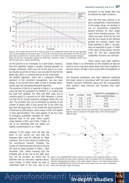
Figure 4: The evolution of the swine flu in Italy according to our modified SIR model. Note that the logarithmic
scale has been adopted for the persons ages. It can be seen that the flu peak falls between the 45th and 46th
week (blue curve)and that it concerns about 13.5 persons out of 1000. The flu should practically disappear
before the new year. The triangles represent the fitted data, contained in Table 1: it immediately becomes clear
that the death rate is slightly overestimated.
of the function to be minimized. It is well known, however,
that this algorithm adopts a penalty oriented approach to
manage constraints, which may not be the best in our case:
we actually would like to have a very accurate fit also for the
death rate, which is involved directly by the constraints.
The NLPQLP algorithm, which has a completely different
approach in the constraint management, has also been
tested: it can be seen (from Table 2) that it provides better
results than the Levenberg-Marquardt algorithm.
The evolution of the flu is reported in Figure 4, as computed
using the best fit parameters by NLPQLP. It is evident that
the peak falls between the 45th and 46th week and it
concerns about 13.5 persons out of 1000. Moreover, it points
out that the flu should practically disappear before the new
year. The mortality rate can be estimated by looking at the
number of deaths after a long period (let us say after one
year from the beginning): in our model this value amounts to
0.0028 out of 1000 persons, which means 0.03% (170 deaths
in Italy approximately). This value appears to be very close
to analogous quantities computed for other
seasonal flues in the past, which usually
range between 0.02% and 0.04%. Finally, it
has to be mentioned that the deaths are
slightly overestimated in our model.
However, if the reader visits the web site
given in [2], he/she can read that the
proposed data could be affected by slight
variations, due to some delays in reporting by
the surveillance network. Probably, the
number of infected persons will not be exactly
the same as those reported in Table 1, after
November 15th. Hence knowing that the
available data at the end of the 46th week
may not be accurate, we would like to
estimate how our previsions reported above,
could change. In other words, we want to
understand what is the error rate of our
Newsletter EnginSoft Year 6 n°4 - 37
previsions, as the target data may
be affected by slight variations.
Here, the first step certainly is to
give a probabilistic characterization
of the target values; we decided to
use an exponential probability
density function for each target
value of the infected persons. This
choice has been driven by the fact
that the true values of the infected
persons are certainly higher than
those reported in Table 1; actually,
they are expected to grow. In Table
3 the values of the location and the
scale for the four exponential
probability functions are collected.
These values have been arbitrary
chosen (there is no information on the reliability of data we
have) in such a way that values lesser than those reported in
the last column of Table 3 have around 90% of probability to
appear.
Five thousand simulations have been organized modifying
the target values in accordance with the given probability
density functions mentioned above and the corresponding
peak position, peak intensity and mortality have been
computed.
Table 3: The location and the scale parameters of the exponential probability
functions used to characterize the target values of the infected people at
different weeks.
Figure 5: The modeFRONTIER workflow used for the solution of the sensitivity problem. A Latin-
Hypercube technique has been used to generate a DOE in accordance with the probability density
functions characterizing the targets. In the project shown in Figure 3, the model tuning problem is
solved by modeFRONTIER with a batch call and a Scilab routine which are used to continuously
extract the information about the disease.