Diffusion Processes with Hidden States from ... - FU Berlin, FB MI

More documents

Recommendations

Info

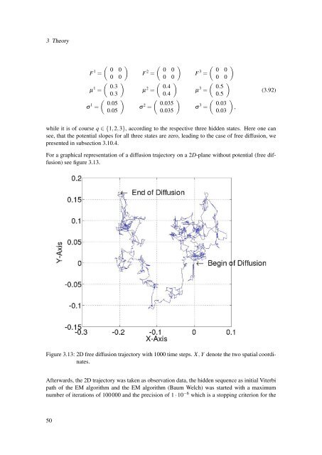
3 Theory( )F 1 0 0=0 0( )µ 1 0.3=0.3( )σ 1 0.05=0.05( ) 0 0F 2 =0 0( ) 0.4µ 2 =0.4( ) 0.035σ 2 =0.035( )F 3 0 0=0 0( )µ 3 0.5=σ 3 =0.5( 0.030.03),(3.92)while it is of course q ∈ {1,2,3}, according to the respective three hidden states. Here one cansee, that the potential slopes for all three states are zero, leading to the case of free diffusion, wepresented in subsection 3.10.4.For a graphical representation of a diffusion trajectory on a 2D-plane without potential (free diffusion)see figure 3.13.Figure 3.13: 2D free diffusion trajectory with 1000 time steps. X, Y denote the two spatial coordinates.Afterwards, the 2D trajectory was taken as observation data, the hidden sequence as initial Viterbipath of the EM algorithm and the EM algorithm (Baum Welch) was started with a maximumnumber of iterations of 100000 and the precision of 1 · 10 −6 which is a stopping criterion for the50
3.12 Artificial Test Examples for Hidden Markov Model - Vector Auto Regression (HMM-VAR)algorithm, meaning that it stops when the change of the new likelihood in comparison with the lastone is not bigger than this number. The algorithm has to be initialized with an initial Viterbi path,in order to get started. We first decided to initialize it with a random sequence of three distinctstates, generated by the same transition matrix, as the sequence which has to be estimated. Thequestion, how the estimation result will be when initializing with a random sequence, created byanother transition matrix, we will investigate later.The procedure of estimation ended after approximately 100 iteration steps. Figure 3.14 shows theconvergence of the likelihood. The estimated transition matrix that we obtained is⎛T est = ⎝0.98 0.01 0.010.01 0.98 0.010.01 0.01 0.98⎞⎠, (3.93)obviously not to distinguish from the true one, given by (3.90).Figure 3.14: Likelihood convergence 1. Convergence of the Likelihood for the estimation of atwo-dimensional trajectory with underlying HMM sequence of 100000 steps.We computed the distance between the two matrices, the true transition matrix (3.90) and theestimated one (3.93) which is equal to the square root of the summed squared distances betweencorresponding entries:51
Page 1:
Diploma ThesisDepartment for Theore
Page 5 and 6:
AbstractAnomalous diffusion is a ub
Page 7 and 8:
Zusammenfassung 1Anomale Diffusion
Page 9 and 10:
Contents1 Motivation 12 Visual Tran
Page 11 and 12: List of Figures2.1 Anatomy of the e
Page 13 and 14: 1 Motivation„NEC FASCES, NEC OPES
Page 15 and 16: Theoretically we profit from enormo
Page 17 and 18: 2 Visual Transduction”The eye owe
Page 19 and 20: (a)(b)(c)Figure 2.3: (a) The anatom
Page 21 and 22: effect of generating the photorecep
Page 23 and 24: 3 Theory”The theory is the net, t
Page 25 and 26: 3.2 Markov Chains, Markov Processes
Page 31 and 32: 3.3 Hidden Markov ModelsP[X(t + τ)
Page 33 and 34: 3.4 Maximum Likelihood Principlewit
Page 35 and 36: 3.5 Optimization3.5 OptimizationAcc
Page 37 and 38: 3.7 Baum-Welch-AlgorithmAlgorithm 3
Page 39 and 40: 3.8 Two Approaches on Stochastic Sy
Page 41 and 42: 3.9 DiffusionConsider a basin fille
Page 43 and 44: 3.9 Diffusion169].Rearranging (3.34
Page 45 and 46: 3.9 Diffusionwith τ = t −t ′ .
Page 47 and 48: 3.9 DiffusionD = 2k2 B T 2σ . (3.4
Page 49 and 50: 3.10 Hidden Markov Models with Stoc
Page 55 and 56: 3.11 Hidden Markov Model - Vector A
Page 57 and 58: 3.11 Hidden Markov Model - Vector A
Page 59 and 60: 3.12 Artificial Test Examples for H
Page 61: 3.12 Artificial Test Examples for H
Page 69 and 70: 3.13 Global Optimization Methods3.1
Page 71 and 72: 3.13 Global Optimization MethodsEve
Page 73 and 74: 4 Fluorescence Tracking Experiments
Page 75 and 76: 4.2 Fluorescence SpectroscopyAfter
Page 77 and 78: 4.3 Single Molecule Tracking via Wi
Page 79 and 80: 4.4 Total Internal Reflection Fluor
Page 81 and 82: 4.4 Total Internal Reflection Fluor
Page 83 and 84: 4.6 The expected range for the Tran
Page 85 and 86: 5 Modeling of the Experiment”The
Page 87 and 88: 5.1 Experimental Data(a)(b)(c)(d)Fi
Page 89 and 90: 5.2 Model Ansatz and Estimation of
Page 91 and 92: 5.2 Model Ansatz and Estimation of
Page 93 and 94: 5.3 Testing the Modelalgorithm was
Page 95 and 96: 5.5 Estimation of the Noise Intensi
Page 97 and 98: 5.6 Estimation on the Basis of Diff
Page 103 and 104: 6 Conclusion and OutlookThe main as
Page 105 and 106: 7 Bibliography[1] R. C. Aster, B. B
Page 107 and 108: [36] C. U. M. Smith: Elements of Mo
Page 109 and 110: Index11-cis retinal isomer, 87TM se
Page 111 and 112: A AppendixA.1 From Copernicus to Ne
Page 113 and 114:
A.2 Important Papers on the Rhodops
Page 115 and 116:
A.3 Probability TheoryDefinition A.
Page 117 and 118:
A.4 Definitions for OptimizationDef
Page 119 and 120:
A.4 Definitions for OptimizationDef
Page 121 and 122:
A.7 The Fluctuation-Dissipation-The
Page 123 and 124:
A.7 The Fluctuation-Dissipation-The
Page 125 and 126:
A.8 Kramers-Moyal Forward Expansion
Page 127 and 128:
A.9 Deriving the Fokker-Planck Equa
Page 129 and 130:
A.9 Deriving the Fokker-Planck Equa
Page 131 and 132:
DanksagungenIch möchte folgenden M
Page 133:
AffirmationHereby I, Arash Azhand,
show all

Diffusion Processes with Hidden States from ... - FU Berlin, FB MI

Create successful ePaper yourself

Delete template?

Save as template?