Diffusion Processes with Hidden States from ... - FU Berlin, FB MI

More documents

Recommendations

Info

5 Modeling of the Experimentsmall amount of data statistically not so relevant, as we wish. But this can be improved, when weobtain more observation data.(a) x-component of the trajectories(b) y-component of the trajectoriesFigure 5.4: Estimation of the noise intensities for single transducin trajectories.In the next section we will present a theoretical formulation of an HMM-VAR estimation frameworkthat is based on observation data consisting of position differences instead of positions, whilethe estimation procedure is identical.84
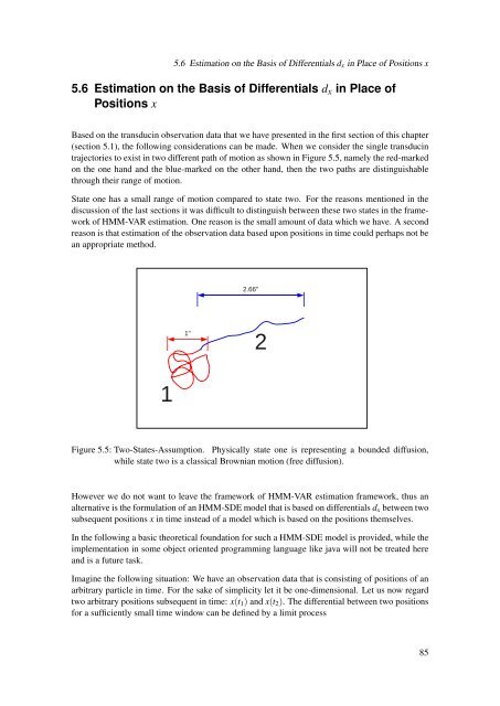
5.6 Estimation on the Basis of Differentials d x in Place of Positions x5.6 Estimation on the Basis of Differentials d x in Place ofPositions xBased on the transducin observation data that we have presented in the first section of this chapter(section 5.1), the following considerations can be made. When we consider the single transducintrajectories to exist in two different path of motion as shown in Figure 5.5, namely the red-markedon the one hand and the blue-marked on the other hand, then the two paths are distinguishablethrough their range of motion.State one has a small range of motion compared to state two. For the reasons mentioned in thediscussion of the last sections it was difficult to distinguish between these two states in the frameworkof HMM-VAR estimation. One reason is the small amount of data which we have. A secondreason is that estimation of the observation data based upon positions in time could perhaps not bean appropriate method.2.66"1"21Figure 5.5: Two-<strong>States</strong>-Assumption. Physically state one is representing a bounded diffusion,while state two is a classical Brownian motion (free diffusion).However we do not want to leave the framework of HMM-VAR estimation framework, thus analternative is the formulation of an HMM-SDE model that is based on differentials d x between twosubsequent positions x in time instead of a model which is based on the positions themselves.In the following a basic theoretical foundation for such a HMM-SDE model is provided, while theimplementation in some object oriented programming language like java will not be treated hereand is a future task.Imagine the following situation: We have an observation data that is consisting of positions of anarbitrary particle in time. For the sake of simplicity let it be one-dimensional. Let us now regardtwo arbitrary positions subsequent in time: x(t 1 ) and x(t 2 ). The differential between two positionsfor a sufficiently small time window can be defined by a limit process85
Page 1:
Diploma ThesisDepartment for Theore
Page 5 and 6:
AbstractAnomalous diffusion is a ub
Page 7 and 8:
Zusammenfassung 1Anomale Diffusion
Page 9 and 10:
Contents1 Motivation 12 Visual Tran
Page 11 and 12:
List of Figures2.1 Anatomy of the e
Page 13 and 14:
1 Motivation„NEC FASCES, NEC OPES
Page 15 and 16:
Theoretically we profit from enormo
Page 17 and 18:
2 Visual Transduction”The eye owe
Page 19 and 20:
(a)(b)(c)Figure 2.3: (a) The anatom
Page 21 and 22:
effect of generating the photorecep
Page 23 and 24:
3 Theory”The theory is the net, t
Page 25 and 26:
3.2 Markov Chains, Markov Processes
Page 27 and 28:
Page 29 and 30:
Page 31 and 32:
3.3 Hidden Markov ModelsP[X(t + τ)
Page 33 and 34:
3.4 Maximum Likelihood Principlewit
Page 35 and 36:
3.5 Optimization3.5 OptimizationAcc
Page 37 and 38:
3.7 Baum-Welch-AlgorithmAlgorithm 3
Page 39 and 40:
3.8 Two Approaches on Stochastic Sy
Page 41 and 42:
3.9 DiffusionConsider a basin fille
Page 43 and 44:
3.9 Diffusion169].Rearranging (3.34
Page 45 and 46: 3.9 Diffusionwith τ = t −t ′ .
Page 47 and 48: 3.9 DiffusionD = 2k2 B T 2σ . (3.4
Page 49 and 50: 3.10 Hidden Markov Models with Stoc
Page 55 and 56: 3.11 Hidden Markov Model - Vector A
Page 57 and 58: 3.11 Hidden Markov Model - Vector A
Page 59 and 60: 3.12 Artificial Test Examples for H
Page 69 and 70: 3.13 Global Optimization Methods3.1
Page 71 and 72: 3.13 Global Optimization MethodsEve
Page 73 and 74: 4 Fluorescence Tracking Experiments
Page 75 and 76: 4.2 Fluorescence SpectroscopyAfter
Page 77 and 78: 4.3 Single Molecule Tracking via Wi
Page 79 and 80: 4.4 Total Internal Reflection Fluor
Page 81 and 82: 4.4 Total Internal Reflection Fluor
Page 83 and 84: 4.6 The expected range for the Tran
Page 85 and 86: 5 Modeling of the Experiment”The
Page 87 and 88: 5.1 Experimental Data(a)(b)(c)(d)Fi
Page 89 and 90: 5.2 Model Ansatz and Estimation of
Page 91 and 92: 5.2 Model Ansatz and Estimation of
Page 93 and 94: 5.3 Testing the Modelalgorithm was
Page 95: 5.5 Estimation of the Noise Intensi
Page 99 and 100: 5.6 Estimation on the Basis of Diff
Page 101 and 102: 5.6 Estimation on the Basis of Diff
Page 103 and 104: 6 Conclusion and OutlookThe main as
Page 105 and 106: 7 Bibliography[1] R. C. Aster, B. B
Page 107 and 108: [36] C. U. M. Smith: Elements of Mo
Page 109 and 110: Index11-cis retinal isomer, 87TM se
Page 111 and 112: A AppendixA.1 From Copernicus to Ne
Page 113 and 114: A.2 Important Papers on the Rhodops
Page 115 and 116: A.3 Probability TheoryDefinition A.
Page 117 and 118: A.4 Definitions for OptimizationDef
Page 119 and 120: A.4 Definitions for OptimizationDef
Page 121 and 122: A.7 The Fluctuation-Dissipation-The
Page 123 and 124: A.7 The Fluctuation-Dissipation-The
Page 125 and 126: A.8 Kramers-Moyal Forward Expansion
Page 127 and 128: A.9 Deriving the Fokker-Planck Equa
Page 129 and 130: A.9 Deriving the Fokker-Planck Equa
Page 131 and 132: DanksagungenIch möchte folgenden M
Page 133: AffirmationHereby I, Arash Azhand,
show all

Diffusion Processes with Hidden States from ... - FU Berlin, FB MI

Create successful ePaper yourself

Delete template?

Save as template?