VLIDORT User's Guide

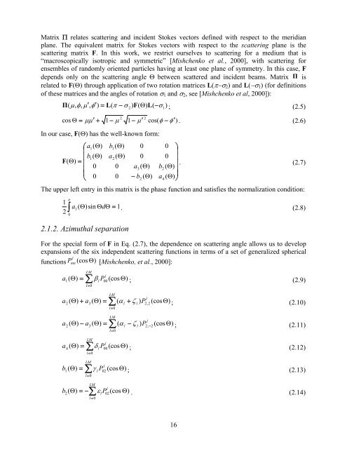
Matrix Π relates scattering and incident Stokes vectors defined with respect to the meridianplane. The equivalent matrix for Stokes vectors with respect to the scattering plane is thescattering matrix F. In this work, we restrict ourselves to scattering for a medium that is“macroscopically isotropic and symmetric” [Mishchenko et al., 2000], with scattering forensembles of randomly oriented particles having at least one plane of symmetry. In this case, Fdepends only on the scattering angle Θ between scattered and incident beams. Matrix Π isrelated to F(Θ) through application of two rotation matrices L(π−σ 2 ) and L(−σ 1 ) (for definitionsof these matrices and the angles of rotation σ 1 and σ 2 , see [Mishchenko et al, 2000]):Π( μ,φ,μ′ , φ′) = L(π − σ 2) F(Θ ) L(−σ1); (2.5)22cos Θ = μ μ′+ 1 − μ 1 − μ ′ cos( φ − φ ′). (2.6)In our case, F(Θ) has the well-known form:⎛ a1(Θ)b1( Θ)0 0 ⎞⎜⎟⎜ b1( Θ)a2( Θ)0 0 ⎟F ( Θ)= ⎜ 0 0 ( ) ( ) ⎟ . (2.7)a3Θ b2Θ⎜⎟⎝ 0 0 − b2( Θ)a4( Θ)⎠The upper left entry in this matrix is the phase function and satisfies the normalization condition:12π∫0a1( Θ)sinΘdΘ= 1. (2.8)2.1.2. Azimuthal separationFor the special form of F in Eq. (2.7), the dependence on scattering angle allows us to developexpansions of the six independent scattering functions in terms of a set of generalized sphericallfunctions Pmn(cos Θ)[Mishchenko, et al., 2000]:LMa = ∑ P l1( )l 00(cos Θ)l=0aaΘ β ; (2.9)LMl2( Θ)+ a3(Θ)= ∑ (l+ ζl) P2,2(cosΘ)l=0α ; (2.10)LMl2( Θ)− a3( Θ)= ∑ (l− ζl) P2,−2(cos Θ)l=0LMa = ∑ P l4( )l 00(cos Θ)l=0α ; (2.11)Θ δ ; (2.12)LMb = ∑ P l1( )l 02(cosΘ)l=0Θ γ ; (2.13)LMb = −∑P l2( )l 02(cosΘ)l = 0Θ ε . (2.14)16