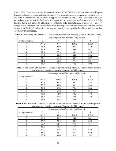
In earlier versions of LIDORT and <strong>VLIDORT</strong>, the converged diffuse field was established first,with the TMS exact scatter term applied afterwards as a correction. Following discussions withMick Christi, it is apparent that an improvement in Fourier convergence can be obtained byapplying TMS first and including I SSexact right from the start in the convergence testing. Therationale here is that the overall field has a larger magnitude with the inclusion of the I SSexactoffset, so that the addition of increasingly smaller Fourier terms will be less of an influence onthe total. This feature has now been installed in <strong>VLIDORT</strong> (Versions 2.1 and higher).It turns out that a similar consideration applies to the direct beam intensity field (the direct solarbeam reflected off the surface, with no atmospheric scattering). For a non-Lambertian surfacewith known BRDF functions, <strong>VLIDORT</strong> will calculated the Fourier contributions from theBRDF terms, and (for the upwelling field) deliver the Fourier components of the post-processeddirect-beam reflection as well as the diffuse and single scatter contributions. The completeFourier-summed direct beam contribution is necessarily truncated because of the discreteordinate process. It is possible to compute an exact BRDF contribution (no Fourier component)for the direct beam, using the original viewing angles, and this I DBexact term will then replacethe truncated contribution I DBtrunc .This feature has now been installed in Versions 2.1 and higher in <strong>VLIDORT</strong> and functions in thesame way as the TMS correction. The truncated form I DBtrunc is simply not calculated and theexact form I DBexact is computed right from the start as an initial correction, and included in theconvergence testing along with the TMS contribution. For sharply peaked strong BRDF surfacecontributions, this “DB correction” can be significant, and may give rise to a substantial savingin Fourier computations, particularly for situations where the atmospheric scattering may bequite well approximated by a low number of discrete ordinates.3.3.7 Enhanced efficiency for observational geometry outputIn 'operational' environments such as satellite atmospheric or surface retrieval algorithms, thereis a common requirement for radiative transfer output at specific “solar zenith angle, viewingangle, relative azimuth angle” observational geometry triplets. Although <strong>VLIDORT</strong> has longhad the capability for multi-geometry output, this facility (in previous versions) was not efficientfor generating output at geometry triplets. For example, if there are 4 triplets, then previously<strong>VLIDORT</strong> was configured to generate 4x4x4=64 output radiation fields, that is, one RT outputfor each of the 4 solar zenith angles, each of the 4 viewing angles, and each of the 4 relativeazimuth angles. One may view this as computing a “4x4x4 lattice cube of solutions”, and this isfine for building a look-up table (LUT). However, out of these 64 values, we require thesolutions along the diagonal of the above “lattice cube of solutions” (i.e. 4 instead of 64, one foreach triplet) for observational output; the other 60 solutions are not needed.To enhance computational performance, <strong>VLIDORT</strong> has been given an observational geometryfacility. This is configured with a Boolean flag, a specific number of geometry triplets and thetriplet angles themselves, and in this situation, a single call to <strong>VLIDORT</strong> will generate thediscrete-ordinate radiation fields for each solar zenith angle for a given triplet, and then carry outpost-processing only for those viewing zenith and relative azimuth angles uniquely associatedwith the triplet solar zenith angles. One of the big time savings here is with the internal geometryroutines in <strong>VLIDORT</strong> - in our example, we require 4 calls instead of 64.Tables 3.3-3.5 indicate the improved efficiency gained by using this observational geometryfeature (“ObsGeo”) for a set of geometries, in lieu of doing a “Lattice” computation for the sameset of geometries. The efficiency in each entry is given as the ratio (ObsGeo time / Lattice50
time)*100%. Tests were made for several values of NSTREAMS (the number of half-spacediscrete ordinates or computational streams). The atmosphere/surface scenario in these tests isthat used in the standard environment wrappers that come with the LIDORT package: a 23-layeratmosphere with aerosol in the lowest six layers and a Lambertian surface (see section 6.2 fordetails). Table 3.3 refers to efficiency of intensity-only computations, whereas in Table 3.4timings were compared for calculations with intensity, two column Jacobians and one surfaceJacobian; in Table 3.5 calculation timings for intensity, three profile Jacobians and one surfaceJacobian were compared.Table 3.3 Efficiency of ObsGeo vs. Lattice computations for intensity (% ratio of CPU values).# of computational streams (half-space)# of geometries 2 4 6 81 101.2 99.7 100.2 100.42 95.4 96.0 98.2 88.63 85.6 88.8 94.0 95.14 72.0 75.9 83.7 87.05 60.0 69.8 84.8 85.66 52.1 68.4 80.7 83.77 41.2 62.8 77.3 82.48 34.3 57.4 73.5 80.8Table 3.4 Efficiency of ObsGeo vs. Lattice computations for intensity, 2 atmospheric columnJacobians and 1 surface Jacobian (% ratio of CPU values).# of computational streams (half-space)# of geometries 2 4 6 81 101.5 100.0 100.1 100.42 90.8 92.3 96.7 88.43 75.7 81.6 86.1 89.44 59.9 66.0 79.4 86.65 46.5 66.0 76.5 81.36 36.0 54.9 70.2 77.97 28.7 47.6 64.6 74.88 23.0 41.5 59.0 71.7Table 3.5 Efficiency of ObsGeo vs. Lattice computations for intensity, 3 atmospheric profileJacobians and 1 surface Jacobian (% ratio of CPU values).# of computational streams (half-space)# of geometries 2 4 6 81 102.7 99.9 100.2 100.32 88.5 88.2 94.0 86.13 73.7 77.3 83.3 83.24 59.7 64.1 71.6 75.75 48.6 55.3 67.4 71.76 39.1 49.6 61.8 67.87 31.7 44.1 57.1 62.98 25.9 39.0 51.8 59.551
- Page 1: User’s GuideVLIDORTVersion 2.6Rob
- Page 5 and 6: Table of Contents1H1. Introduction
- Page 7 and 8: 1. Introduction to VLIDORT1.1. Hist
- Page 9 and 10: Table 1.1 Major features of LIDORT
- Page 11 and 12: In 2006, R. Spurr was invited to co
- Page 13: corrections, and sphericity correct
- Page 16 and 17: Matrix Π relates scattering and in
- Page 18 and 19: m⎛ P⎞l( μ)0 0 0⎜⎟mmm ⎜ 0
- Page 20 and 21: In the following sections, we suppr
- Page 22 and 23: of the single scatter albedo ω and
- Page 24 and 25: Here T n−1 is the solar beam tran
- Page 26 and 27: ~ + ~ ~ (1)~ ~ + ~ ~ (2)~ ~ − ~ 1
- Page 28 and 29: The solution proceeds first by the
- Page 30 and 31: Linearizations. Derivatives of all
- Page 32 and 33: For the plane-parallel case, we hav
- Page 34 and 35: One of the features of the above ou
- Page 36 and 37: L↑↑ ↑k (cot n −cotn −1)[
- Page 38 and 39: Note the use of the profile-column
- Page 40 and 41: βl,aer(1)(2)fz1e1βl+ ( 1−f ) z2
- Page 42 and 43: For BRDF input, it is necessary for
- Page 44 and 45: streams were used in the half space
- Page 46 and 47: anded tri-diagonal matrix A contain
- Page 48 and 49: in place to aid with the LU-decompo
- Page 53 and 54: 4. The VLIDORT 2.6 package4.1. Over
- Page 55 and 56: (discrete ordinates), so that dimen
- Page 57 and 58: Table 4.2 Summary of VLIDORT I/O Ty
- Page 59 and 60: Table 4.3. Module files in VLIDORT
- Page 61 and 62: Finally, modules vlidort_ls_correct
- Page 63 and 64: end program main_VLIDORT4.3.2. Conf
- Page 65 and 66: $(VLID_DEF_PATH)/vlidort_sup_brdf_d
- Page 67 and 68: Finally, the command to build the d
- Page 69 and 70: Here, “s” indicates you want to
- Page 71 and 72: The main difference between “vlid
- Page 73 and 74: to both VLIDORT and the given VSLEA
- Page 75 and 76: STATUS_INPUTREAD is equal to 4 (VLI
- Page 77 and 78: 5. ReferencesAnderson, E., Z. Bai,
- Page 79 and 80: Mishchenko, M.I., and L.D. Travis,
- Page 81: Stamnes K., S-C. Tsay, W. Wiscombe,
- Page 84 and 85: Table A2: Type Structure VLIDORT_Fi
- Page 86 and 87: DO_WRITE_FOURIER Logical (I) Flag f
- Page 88 and 89: USER_LEVELS (o) Real*8 (IO) Array o
- Page 90 and 91: angle s, Stokes parameter S, and di
- Page 92 and 93: DO_SLEAVE_WFS Logical (IO) Flag for
- Page 94 and 95: 6.1.1.8. VLIDORT linearized outputs
- Page 96 and 97: NFINELAYERS Integer Number of fine
- Page 98 and 99: 6.1.2.4. VLIDORT linearized modifie
- Page 100 and 101:
The output file contains (for all 3
- Page 102 and 103:
The first call is the baseline calc
- Page 104 and 105:
for a 2-parameter Gamma-function si
- Page 106 and 107:
Remark. In VLIDORT, the BRDF is a 4
- Page 108 and 109:
6.3.3.1. Input and output type stru
- Page 110 and 111:
Table C: Type Structure VBRDF_LinSu
- Page 112 and 113:
Special note regarding Cox-Munk typ
- Page 114 and 115:
squared parameter, so that Jacobian
- Page 116 and 117:
6.4. SLEAVE SupplementHere, the sur
- Page 118 and 119:
is possible to define Jacobians wit
- Page 120 and 121:
etween 0 and 90 degrees.N_USER_OBSG
- Page 122:
6.4.4.2 SLEAVE configuration file c