VLIDORT User's Guide

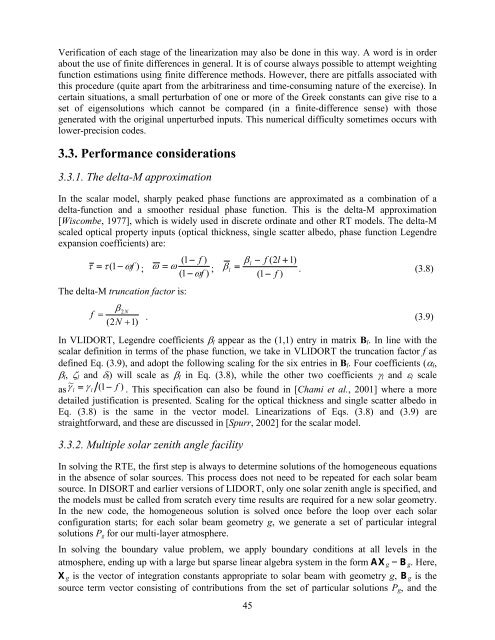
Verification of each stage of the linearization may also be done in this way. A word is in orderabout the use of finite differences in general. It is of course always possible to attempt weightingfunction estimations using finite difference methods. However, there are pitfalls associated withthis procedure (quite apart from the arbitrariness and time-consuming nature of the exercise). Incertain situations, a small perturbation of one or more of the Greek constants can give rise to aset of eigensolutions which cannot be compared (in a finite-difference sense) with thosegenerated with the original unperturbed inputs. This numerical difficulty sometimes occurs withlower-precision codes.3.3. Performance considerations3.3.1. The delta-M approximationIn the scalar model, sharply peaked phase functions are approximated as a combination of adelta-function and a smoother residual phase function. This is the delta-M approximation[Wiscombe, 1977], which is widely used in discrete ordinate and other RT models. The delta-Mscaled optical property inputs (optical thickness, single scatter albedo, phase function Legendreexpansion coefficients) are:τ = τ ( 1−ωf) ;(1 − f )ω = ω(1 − ωf);The delta-M truncation factor is:β2Nf =(2N+ 1)l− f (2l+ 1)βl= β. (3.8)(1 − f ). (3.9)In VLIDORT, Legendre coefficients β l appear as the (1,1) entry in matrix B l . In line with thescalar definition in terms of the phase function, we take in VLIDORT the truncation factor f asdefined Eq. (3.9), and adopt the following scaling for the six entries in B l . Four coefficients (α l ,β l , ζ l and δ l ) will scale as β l in Eq. (3.8), while the other two coefficients γ l and ε l scale~as γl= γl(1 − f ) . This specification can also be found in [Chami et al., 2001] where a moredetailed justification is presented. Scaling for the optical thickness and single scatter albedo inEq. (3.8) is the same in the vector model. Linearizations of Eqs. (3.8) and (3.9) arestraightforward, and these are discussed in [Spurr, 2002] for the scalar model.3.3.2. Multiple solar zenith angle facilityIn solving the RTE, the first step is always to determine solutions of the homogeneous equationsin the absence of solar sources. This process does not need to be repeated for each solar beamsource. In DISORT and earlier versions of LIDORT, only one solar zenith angle is specified, andthe models must be called from scratch every time results are required for a new solar geometry.In the new code, the homogeneous solution is solved once before the loop over each solarconfiguration starts; for each solar beam geometry g, we generate a set of particular integralsolutions P g for our multi-layer atmosphere.In solving the boundary value problem, we apply boundary conditions at all levels in theatmosphere, ending up with a large but sparse linear algebra system in the form AX g = B g . Here,X g is the vector of integration constants appropriate to solar beam with geometry g, B g is thesource term vector consisting of contributions from the set of particular solutions P g , and the45