VLIDORT User's Guide

More documents

Recommendations

Info

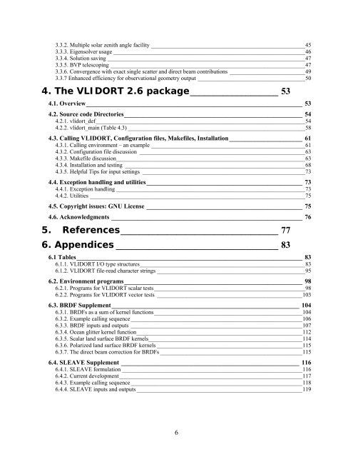
52H4. The68H5. References__________________________________69H6. Appendices46H3.3.2. Multiple solar zenith angle facility _____________________________________________________ 135H4547H3.3.3. Eigensolver usage __________________________________________________________________ 136H4648H3.3.4. Solution saving ____________________________________________________________________ 137H4749H3.3.5. BVP telescoping ___________________________________________________________________ 138H4750H3.3.6. Convergence with exact single scatter and direct beam contributions __________________________ 139H4951H3.3.7 Enhanced efficiency for observational geometry output _____________________________________ 140H50VLIDORT 2.6 package___________________ 141H5353H4.1. Overview____________________________________________________________________ 142H5354H4.2. Source code Directories________________________________________________________ 143H5455H4.2.1. vlidort_def________________________________________________________________________ 144H5456H4.2.2. vlidort_main (Table 4.3) _____________________________________________________________ 145H5857H4.3. Calling VLIDORT, Configuration files, Makefiles, Installation _______________________ 146H6158H4.3.1. Calling environment – an example _____________________________________________________ 147H6159H4.3.2. Configuration file discussion _________________________________________________________ 148H6360H4.3.3. Makefile discussion_________________________________________________________________ 149H6361H4.3.4. Installation and testing ______________________________________________________________ 150H6862H4.3.5. Helpful Tips for input settings ________________________________________________________ 151H7363H4.4. Exception handling and utilities_________________________________________________ 152H7364H4.4.1. Exception handling _________________________________________________________________ 153H7365H4.4.2. Utilities __________________________________________________________________________ 154H7566H4.5. Copyright issues: GNU License _________________________________________________ 155H7567H4.6. Acknowledgments ____________________________________________________________ 156H76157H77___________________________________ 158H8370H6.1 Tables_______________________________________________________________________ 159H8371H6.1.1. VLIDORT I/O type structures_________________________________________________________ 160H8372H6.1.2. VLIDORT file-read character strings ___________________________________________________ 161H9573H6.2. Environment programs________________________________________________________ 162H9874H6.2.1. Programs for VLIDORT scalar tests____________________________________________________ 163H9875H6.2.2. Programs for VLIDORT vector tests __________________________________________________ 164H10376H6.3. BRDF Supplement___________________________________________________________ 165H10477H6.3.1. BRDFs as a sum of kernel functions___________________________________________________ 166H10478H6.3.2. Example calling sequence ___________________________________________________________ 167H10679H6.3.3. BRDF inputs and outputs ___________________________________________________________ 168H10780H6.3.4. Ocean glitter kernel function_________________________________________________________ 169H11281H6.3.5. Scalar land surface BRDF kernels_____________________________________________________ 170H11482H6.3.6. Polarized land surface BRDF kernels __________________________________________________ 171H11583H6.3.7. The direct beam correction for BRDFs _________________________________________________ 172H11584H6.4. SLEAVE Supplement ________________________________________________________ 173H11685H6.4.1. SLEAVE formulation ______________________________________________________________ 174H11686H6.4.2. Current development_______________________________________________________________ 175H11787H6.4.3. Example calling sequence ___________________________________________________________ 176H11888H6.4.4. SLEAVE inputs and outputs _________________________________________________________ 177H1196
1. Introduction to VLIDORT1.1. Historical and background overview1.1.1. Polarization in radiative transferThe modern treatment of the equations of radiative transfer for polarized light dates back to thepioneering work by Chandrasekhar in the 1940s [Chandrasekhar, 1960]. Using a formulation interms of the Stokes vector for polarized light, Chandrasekhar was able to solve completely thepolarization problem for an atmosphere with Rayleigh scattering, and benchmark calculationsfrom the 1950s are still appropriate today [Coulson et al., 1960]. Researchers started looking atthe scattering properties of polarized light by particles, and new more general formulations of thescattering matrices were developed independently by Hovenier [Hovenier, 1971] and Dave[Dave, 1970], and subsequently used in studies of polarization by Venus.With the advent of more powerful computers, a series of numerical RTMs were developedthrough the 1980s; many of these have become standards. In particular, the DISORT discreteordinate model developed by Stamnes and co-workers was released in 1988 for general use[Stamnes, et al., 1988]. Most RTMs today are either discrete ordinate codes or doubling-addingmethods, and vector models are no exception. In the 1980s, Siewert and colleagues made anumber of detailed mathematical examinations of the vector RT equations. The development ofthe scattering matrix in terms of generalized spherical functions was reformulated in aconvenient analytic manner [Siewert, 1981; Siewert, 1982; Vestrucci and Siewert, 1984], andmost models now follow this work (this includes VLIDORT). Siewert and co-workers thencarried out an examination of the discrete ordinate eigenspectrum for the vector equations, anddeveloped complete solutions for the slab problem using the spherical harmonics method[Garcia and Siewert, 1986] and the F N method [Garcia and Siewert, 1989]. These last twosolutions have generated benchmark results for the slab problem.Also in the 1980s, a group in the Netherlands carried out some parallel developments. Followingdetailed mathematical studies by Hovenier and others [Hovenier and van der Mee, 1983; deRooij and van der Stap, 1984], a general doubling-adding model was developed for atmosphericradiative transfer modeling [de Haan et al., 1987; Stammes et al., 1989]. This group was alsoable to provide benchmark results for the slab problem [Wauben and Hovenier, 1992]. Vectordiscrete ordinate models were developed in the 1990s, with VDISORT [Schultz et al., 2000] andits generalization [Schultz and Stamnes, 2000] to include the post processing function. In 1998,Siewert revisited the slab problem from a discrete ordinate viewpoint, and developed new andelegant solutions for the scalar [Siewert, 2000a] and vector [Siewert, 2000b] problems. One newingredient in these solutions was the use of Green’s functions to develop particular solutions forthe solar scattering term [Barichello et al., 2000]. For the vector problem, Siewert’s analysisshowed that complex eigensolutions for the homogeneous RT equations must be considered.Siewert also provided a new set of benchmark results [Siewert, 2000b]; this set and the resultsfrom [Garcia and Siewert, 1989] constitute our standards for slab-problem validation withaerosols.7
Page 1: User’s GuideVLIDORTVersion 2.6Rob
Page 5: Table of Contents1H1. Introduction
Page 9 and 10: Table 1.1 Major features of LIDORT
Page 11 and 12: In 2006, R. Spurr was invited to co
Page 13: corrections, and sphericity correct
Page 16 and 17: Matrix Π relates scattering and in
Page 18 and 19: m⎛ P⎞l( μ)0 0 0⎜⎟mmm ⎜ 0
Page 20 and 21: In the following sections, we suppr
Page 22 and 23: of the single scatter albedo ω and
Page 24 and 25: Here T n−1 is the solar beam tran
Page 26 and 27: ~ + ~ ~ (1)~ ~ + ~ ~ (2)~ ~ − ~ 1
Page 28 and 29: The solution proceeds first by the
Page 30 and 31: Linearizations. Derivatives of all
Page 32 and 33: For the plane-parallel case, we hav
Page 34 and 35: One of the features of the above ou
Page 36 and 37: L↑↑ ↑k (cot n −cotn −1)[
Page 38 and 39: Note the use of the profile-column
Page 40 and 41: βl,aer(1)(2)fz1e1βl+ ( 1−f ) z2
Page 42 and 43: For BRDF input, it is necessary for
Page 44 and 45: streams were used in the half space
Page 46 and 47: anded tri-diagonal matrix A contain
Page 48 and 49: in place to aid with the LU-decompo
Page 50 and 51: In earlier versions of LIDORT and V
Page 53 and 54: 4. The VLIDORT 2.6 package4.1. Over
Page 55 and 56: (discrete ordinates), so that dimen
Page 57 and 58:
Table 4.2 Summary of VLIDORT I/O Ty
Page 59 and 60:
Table 4.3. Module files in VLIDORT
Page 61 and 62:
Finally, modules vlidort_ls_correct
Page 63 and 64:
end program main_VLIDORT4.3.2. Conf
Page 65 and 66:
$(VLID_DEF_PATH)/vlidort_sup_brdf_d
Page 67 and 68:
Finally, the command to build the d
Page 69 and 70:
Here, “s” indicates you want to
Page 71 and 72:
The main difference between “vlid
Page 73 and 74:
to both VLIDORT and the given VSLEA
Page 75 and 76:
STATUS_INPUTREAD is equal to 4 (VLI
Page 77 and 78:
5. ReferencesAnderson, E., Z. Bai,
Page 79 and 80:
Mishchenko, M.I., and L.D. Travis,
Page 81:
Stamnes K., S-C. Tsay, W. Wiscombe,
Page 84 and 85:
Table A2: Type Structure VLIDORT_Fi
Page 86 and 87:
DO_WRITE_FOURIER Logical (I) Flag f
Page 88 and 89:
USER_LEVELS (o) Real*8 (IO) Array o
Page 90 and 91:
angle s, Stokes parameter S, and di
Page 92 and 93:
DO_SLEAVE_WFS Logical (IO) Flag for
Page 94 and 95:
6.1.1.8. VLIDORT linearized outputs
Page 96 and 97:
NFINELAYERS Integer Number of fine
Page 98 and 99:
6.1.2.4. VLIDORT linearized modifie
Page 100 and 101:
The output file contains (for all 3
Page 102 and 103:
The first call is the baseline calc
Page 104 and 105:
for a 2-parameter Gamma-function si
Page 106 and 107:
Remark. In VLIDORT, the BRDF is a 4
Page 108 and 109:
6.3.3.1. Input and output type stru
Page 110 and 111:
Table C: Type Structure VBRDF_LinSu
Page 112 and 113:
Special note regarding Cox-Munk typ
Page 114 and 115:
squared parameter, so that Jacobian
Page 116 and 117:
6.4. SLEAVE SupplementHere, the sur
Page 118 and 119:
is possible to define Jacobians wit
Page 120 and 121:
etween 0 and 90 degrees.N_USER_OBSG
Page 122:
6.4.4.2 SLEAVE configuration file c
show all

VLIDORT User's Guide

You also want an ePaper? Increase the reach of your titles

Delete template?

Save as template?