VLIDORT User's Guide

More documents

Recommendations

Info

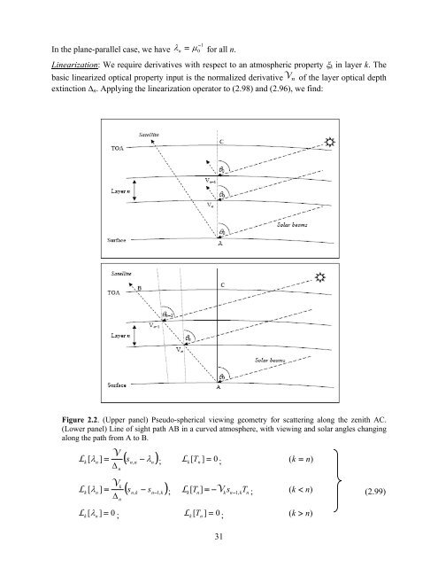
Linearizations. Derivatives of all these expressions may be determined by differentiation withrespect to variable ξ n in layer n. The end-points of the chain rule differentiation are the linearizedoptical property inputs { Vn , U n, Z nl} from Eq. (2.33). For linearization of the homogeneous postprocessingsource term in layer n, there is no dependency on any quantities outside of layer n; in−other words, Lp[ H n( x,μ)]≡ 0 for p ≠ n. The particular solution post-processing source terms inlayer n depend on optical thickness values in all layers above and equal to n through the presenceof the average secant and the solar beam transmittances, so there will be cross-layer derivatives.However, the chain-rule differentiation method is the same, and requires a careful exercise inalgebraic manipulation.Multiplier expressions (2.89), (2.90) and (2.92) have appeared a number of times in theliterature. The linearizations were discussed in [Spurr, 2002] and [Van Oss and Spurr, 2002], andwe need only make two remarks here. Firstly, the real and complex homogeneous solutionmultipliers are treated separately, with the real part of the complex variable result to be used inthe final reckoning. Second, the solar source term multipliers (for example in Eq. (2.92) are thesame as those in the scalar model.Linearizations of the thermal post-processed solution are straightforward; details for the scalarsolution in LIDORT were noted in the review paper [Spurr, 2008].2.4. Spherical and single-scatter corrections in LIDORT2.4.1. Pseudo-spherical approximationThe pseudo-spherical (P-S) approximation assumes solar beam attenuation for a curvedatmosphere. All scattering takes place in a plane-parallel situation. The approximation is astandard feature of many radiative transfer models. We follow the formulation in [Spurr, 2002].Figure 2.2 provides geometrical sketches appropriate to this section.We consider a stratified atmosphere of optically uniform layers, with extinction optical depths{Δ n }, n = 1, N TOTAL (the total number of layers). We take points V n−1 and V n on the vertical(Figure 1, upper panel), and the respective solar beam transmittances to these points are then:n⎡ ⎤= ⎢ − ∑ − 1n⎡ ⎤Tn−1exp s n −1,kΔ k ⎥ ; T n = exp⎢− ∑ s n , kΔk ⎥⎦ . (2.96)⎣ k=1 ⎦⎣ k = 1Here, s n,k is the path distance geometrical factor (Chapman factor), equal to the path distancecovered by the V n beam as it traverses through layer k divided by the corresponding verticalheight drop (geometrical thickness of layer k). At the top of the atmosphere, T0= 1 . In theaverage secant parameterization, the transmittance to any intermediate point between V n−1 and V nis parameterized by:T ( x ) = T exp n−1 [ − λnx], (2.97)where x is the vertical optical thickness measured downwards from V n−1 and λ n the averagesecant for this layer. Substituting (2.97) into (2.96) and setting x = Δ n we find:nn−11 ⎡⎤λn= ⎢∑sn,kΔk− ∑ sn−1, kΔk ⎥ . (2.98)Δn ⎣ k=1k=1 ⎦30
1In the plane-parallel case, we have λ = μ−n 0 for all n.Linearization: We require derivatives with respect to an atmospheric property ξ k in layer k. Thebasic linearized optical property input is the normalized derivativeV n of the layer optical depthextinction Δ n . Applying the linearization operator to (2.98) and (2.96), we find:Figure 2.2. (Upper panel) Pseudo-spherical viewing geometry for scattering along the zenith AC.(Lower panel) Line of sight path AB in a curved atmosphere, with viewing and solar angles changingalong the path from A to B.( − )VL ; L [ ] = 0 ; ( k = n)k[ λn] = sn,nλnΔn( − s )kk[n] sn,k n−1,knkT nVL λ = ; Lk[ Tn]= −Vksn−1,kTn; ( k < n)(2.99)ΔL [ ] = 0 ; L [ ] = 0 ; ( k > n)kλ nkT n31
Page 1: User’s GuideVLIDORTVersion 2.6Rob
Page 5 and 6: Table of Contents1H1. Introduction
Page 7 and 8: 1. Introduction to VLIDORT1.1. Hist
Page 9 and 10: Table 1.1 Major features of LIDORT
Page 11 and 12: In 2006, R. Spurr was invited to co
Page 13: corrections, and sphericity correct
Page 16 and 17: Matrix Π relates scattering and in
Page 18 and 19: m⎛ P⎞l( μ)0 0 0⎜⎟mmm ⎜ 0
Page 20 and 21: In the following sections, we suppr
Page 22 and 23: of the single scatter albedo ω and
Page 24 and 25: Here T n−1 is the solar beam tran
Page 26 and 27: ~ + ~ ~ (1)~ ~ + ~ ~ (2)~ ~ − ~ 1
Page 28 and 29: The solution proceeds first by the
Page 32 and 33: For the plane-parallel case, we hav
Page 34 and 35: One of the features of the above ou
Page 36 and 37: L↑↑ ↑k (cot n −cotn −1)[
Page 38 and 39: Note the use of the profile-column
Page 40 and 41: βl,aer(1)(2)fz1e1βl+ ( 1−f ) z2
Page 42 and 43: For BRDF input, it is necessary for
Page 44 and 45: streams were used in the half space
Page 46 and 47: anded tri-diagonal matrix A contain
Page 48 and 49: in place to aid with the LU-decompo
Page 50 and 51: In earlier versions of LIDORT and V
Page 53 and 54: 4. The VLIDORT 2.6 package4.1. Over
Page 55 and 56: (discrete ordinates), so that dimen
Page 57 and 58: Table 4.2 Summary of VLIDORT I/O Ty
Page 59 and 60: Table 4.3. Module files in VLIDORT
Page 61 and 62: Finally, modules vlidort_ls_correct
Page 63 and 64: end program main_VLIDORT4.3.2. Conf
Page 65 and 66: $(VLID_DEF_PATH)/vlidort_sup_brdf_d
Page 67 and 68: Finally, the command to build the d
Page 69 and 70: Here, “s” indicates you want to
Page 71 and 72: The main difference between “vlid
Page 73 and 74: to both VLIDORT and the given VSLEA
Page 75 and 76: STATUS_INPUTREAD is equal to 4 (VLI
Page 77 and 78: 5. ReferencesAnderson, E., Z. Bai,
Page 79 and 80: Mishchenko, M.I., and L.D. Travis,
Page 81:
Stamnes K., S-C. Tsay, W. Wiscombe,
Page 84 and 85:
Table A2: Type Structure VLIDORT_Fi
Page 86 and 87:
DO_WRITE_FOURIER Logical (I) Flag f
Page 88 and 89:
USER_LEVELS (o) Real*8 (IO) Array o
Page 90 and 91:
angle s, Stokes parameter S, and di
Page 92 and 93:
DO_SLEAVE_WFS Logical (IO) Flag for
Page 94 and 95:
6.1.1.8. VLIDORT linearized outputs
Page 96 and 97:
NFINELAYERS Integer Number of fine
Page 98 and 99:
6.1.2.4. VLIDORT linearized modifie
Page 100 and 101:
The output file contains (for all 3
Page 102 and 103:
The first call is the baseline calc
Page 104 and 105:
for a 2-parameter Gamma-function si
Page 106 and 107:
Remark. In VLIDORT, the BRDF is a 4
Page 108 and 109:
6.3.3.1. Input and output type stru
Page 110 and 111:
Table C: Type Structure VBRDF_LinSu
Page 112 and 113:
Special note regarding Cox-Munk typ
Page 114 and 115:
squared parameter, so that Jacobian
Page 116 and 117:
6.4. SLEAVE SupplementHere, the sur
Page 118 and 119:
is possible to define Jacobians wit
Page 120 and 121:
etween 0 and 90 degrees.N_USER_OBSG
Page 122:
6.4.4.2 SLEAVE configuration file c
show all

VLIDORT User's Guide

Create successful ePaper yourself

Delete template?

Save as template?