Bath Institute For Complex Systems - ENS de Cachan - Antenne de ...
Bath Institute For Complex Systems - ENS de Cachan - Antenne de ...
Bath Institute For Complex Systems - ENS de Cachan - Antenne de ...

Create successful ePaper yourself
Turn your PDF publications into a flip-book with our unique Google optimized e-Paper software.
Corollary 3.10. Let Assumptions A1–A4 hold, for some 0 < t < 1 and p ∗ ∈ (0, ∞]. Then, for allp < p ∗ , s < t with s ≠ 1/2 and h > 0, we have‖u − u h ‖ L p (Ω,L 2 (D)) C 3.10 ‖f‖ L p∗(Ω,H s−1 (D)) h 2s amax‖a‖ 7/2 2 C, where C 3.10 :=t (D)∥∥with q = p∗ pp ∗−p. If Assumptions A2 and A3 hold with t = 1, then‖u − u h ‖ L p (Ω,L 2 (D)) C 3.10 ‖f‖ L p∗(Ω,L 2 (D)) h 2 .a 13/2min∥L q (Ω)Proof. We will use a duality argument. <strong>For</strong> almost all ω ∈ Ω, let e ω := u(ω, ·)−u h (ω, ·) and <strong>de</strong>noteby w ω the solution to the adjoint problemb ω (v, w ω ) = (e ω , v)for all v ∈ H 1 0 (D),which, by Proposition 3.1 with f(ω, ·) = e ω , is also in H 1+s (D). By Galerkin orthogonality‖e ω ‖ 2 L 2 (D) = (e ω, e ω ) L 2 (D) = b ω (e ω , w ω − z h ), for any z h ∈ V h .Using the boun<strong>de</strong>dness of b ω (·, ·) and Lemma 3.7, we then get‖e ω ‖ 2 L 2 (D) a max(ω) |u(ω, ·) − u h (ω, ·)| H 1 (D) ‖w ω ‖ H 1+s (D) h s .Now it follows from Proposition 3.1 and Theorem 3.9 that‖e ω ‖ 2 L 2 (D) ≤ a max(ω) C 3.1 (ω) 2 C 3.8 (ω) ‖f(ω, ·)‖ H s−1 (D)‖e ω ‖ L 2 (D) h 2s .Dividing by ‖e ω ‖ L 2 (D), the result follows again by an application of Höl<strong>de</strong>r’s inequality.Remark 3.11. As usual, the analysis can be exten<strong>de</strong>d in a straightforward way to other boundaryconditions, to tensor coefficients, or to more complicated PDEs including low–or<strong>de</strong>r terms, provi<strong>de</strong>dthe boundary data and the coefficients are sufficiently regular, see [18] for <strong>de</strong>tails.3.3 Quadrature ErrorThe integrals appearing in the bilinear form∑∫b ω (w h , v h ) =a(ω, x)∇w h · ∇v h dxττ∈T h : τ∈D hand in the linear functional L ω (v h ) involve realisations of random fields. It will in general beimpossible to evaluate these integrals exactly, and so we will use quadrature instead. We will onlyexplicitly analyse the quadrature error in b ω , but the quadrature error in approximating L ω (v h )can be analysed analogously.In our analysis, we use the midpoint rule, approximating the integrand by its value at themidpoint x τ of each simplex τ ∈ T h . The trapezoidal rule which we use in the numerical sectioncan be analysed analogously. Let us <strong>de</strong>note the resulting bilinear form that approximates b ω onthe grid T h by∑∫˜bω (w h , v h ) = a(ω, x τ ) ∇w h (x) · ∇v h (x) dx ,ττ∈T h : τ∈D hand let ũ h (ω, ·) <strong>de</strong>note the corresponding solution to˜bω (ũ h (ω, ·), v h ) = L ω (v h ) , for all v h ∈ V h .Clearly the bilinear form ˜b ω is boun<strong>de</strong>d and coercive, with the same constants as the exactbilinear form b ω and so we can apply the following classical result [6] (with explicit <strong>de</strong>pen<strong>de</strong>nce ofthe bound on the coefficients).12