Bath Institute For Complex Systems - ENS de Cachan - Antenne de ...

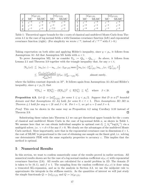
|u| H 1 (D)‖u‖ L 2 (D)|u| H 13 ε −5 ε −3 ε −7/2 ε −2 3 ε −8 ε −6 ε −5 ε −3‖u‖ L 2 (D)d MC MLMC MC MLMC d MC(D)MLMC MC MLMC1 ε −3 ε −2 ε −5/2 ε −2 1 ε −4 ε −2 ε −3 ε −22 ε −4 ε −2 ε −3 ε −2 2 ε −6 ε −4 ε −4 ε −2Table 1: Theoretical upper bounds for the ε-costs of classical and multilevel Monte Carlo from Theorem4.1 in the case of log-normal fields a with Gaussian covariance function (left) and exponentialcovariance function (right). (For simplicity we wrote ε −p , instead of ε −p−δ with δ > 0.)Taking expectation on both sides and applying Hölder’s inequality, since q < p ∗ , it follows fromAssumptions A1–A3 that Assumption M1 holds with α < t.To prove Assumption M2, let us consider Y hl := Q hl − Q hl−1 . As above, it follows fromLemma 2.1 and Theorem 3.9 together with the triangle inequality that, for any s < t,{}|Y hl (ω)| |u hl (ω, ·) − u hl−1 (ω, ·)| H 1 (D) max |u hl (ω, ·)| q−1H 1 (D) , |u h l−1(ω, ·)| q−1H 1 (D) , 1 C 3.1(ω) C 3.8 (ω)a q−1min (ω) ‖f(ω, ·)‖ q H s−1 (D) hs l , almost surely,where the hidden constant depends on M ∗ . It follows again from Assumptions A1-A3 and Hölder’sinequality, since q < p ∗ /2, thatV[Y hl ] = E[Yh 2 l] − (E[Y hl ]) 2 ≤ E[Yh 2 l] h β l, where β < 2t.Proposition 4.3. Let Q := ‖u‖ q L 2 (D) , for some 1 ≤ q < p ∗/2. Suppose that D is a C 2 boundeddomain and that Assumptions A1–A4 hold, for some 0 < t < 1. Then Assumptions M1–M2 inTheorem 4.1 hold for any α < 2t and β < 4t. For t = 1, we get α = 2 and β = 4.Proof. This can be shown in the same way as Proposition 4.2 using Corollary 3.10 instead ofTheorem 3.9.Substituting these values into Theorem 4.1 we can get theoretical upper bounds for the ε-costsof classical and multilevel Monte Carlo in the case of log-normal fields a, as shown in Table 1.We assume here that we can obtain individual samples in optimal cost C l h −dllog(h −1l) via amultigrid solver, i.e. γ = d+δ for any δ > 0. We clearly see the advantages of the multilevel MonteCarlo method. More importantly, note that in the exponential covariance case in dimensions d > 1,the cost of MLMC is proportional to the cost of obtaining one sample on the finest grid, i.e. solvingone deterministic PDE with the same regularity properties to accuracy ε. This implies that themethod is optimal.5 Numerical ResultsIn this section, we want to confirm numerically some of the results proved in earlier sections. Allnumerical results shown are for the case of a log-normal random coefficient a(ω, x) with exponentialcovariance function (2.6). All results are calculated for a model problem in 1D. The domain Dis taken to be (0, 1), and f ≡ 1. The sampling from the random coefficient a(ω, x) is done usinga truncated KL-expansion, and as in the analysis in Section 3.3, we use the midpoint rule toapproximate the integrals in the stiffness matrix. As the quantities of interest we will just studythe simple functionals Q := ‖u‖ L 2 (D) and Q := |u| H 1 (D).17