Bath Institute For Complex Systems - ENS de Cachan - Antenne de ...

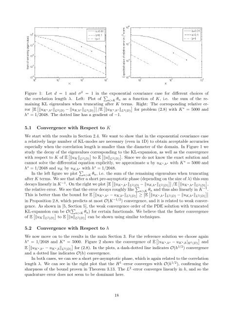
Figure 1: Let d = 1 and σ 2 = 1 in the exponential covariance case for different choices ofthe correlation length λ. Left: Plot of ∑ n>K θ n as a function of K, i.e. the sum of the remainingKL eigenvalues when truncating after K terms. Right: The corresponding relative error∣ ∣E [ ‖u K ∗ ,h ∗‖ L 2 (D) − ‖u K,h ∗‖ L 2 (D)]∣∣ /E [ ‖u K ∗ ,h ∗‖ L 2 (D)]for problem (2.8) with K ∗ = 5000 andh ∗ = 1/2048. The dotted line has a gradient of −1.5.1 Convergence with Respect to KWe start with the results in Section 2.4. We want to show that in the exponential covariance casea relatively large number of KL-modes are necessary (even in 1D) to obtain acceptable accuraciesespecially when the correlation length is smaller than the diameter of the domain. In Figure 1 westudy the decay of the eigenvalues corresponding to the KL-expansion, as well as the convergencewith respect to K of E [ [‖u K ‖ L (D)] 2 to E ‖u‖L (D)] 2 . Since we do not know the exact solution andcannot solve the differential equation explicitly, we approximate u by u K ∗ ,h ∗ with K∗ = 5000 andh ∗ = 1/2048 and u K by u K,h ∗ with h ∗ = 1/2048.In the left figure we plot ∑ n>K θ n, i.e. the sum of the remaining eigenvalues when truncatingafter K terms. We see that after a short pre-asymptotic phase (depending on the size of λ) this sumdecays linearly in K −1 . On the right we plot ∣ ∣E [ ‖u K ∗ ,h ∗‖ L 2 (D) − ‖u K,h ∗‖ L (D)]∣∣ 2 /E [ ‖u K ∗ ,h ∗‖ L (D)] 2 ,the relative error. We see that the error decays roughly like ∑ n>K θ n and thus also linearly in K −1 .This is better than the bound for E [ ‖u K ∗ ,h ∗ − u K,h ∗‖ ∣L (D)] 2 ≥ E [ ‖u K ∗ ,h ∗‖ L 2 (D) − ‖u K,h ∗‖ L (D)]∣∣2in Proposition 2.8, which predicts at most O(K −1/2 ) convergence, and it is related to weak convergence.As shown in [5, Section 5], the weak convergence order of the PDE solution with truncatedKL-expansion can be O( ∑ n>K θ n) for certain functionals. We believe that the faster convergenceof E [ [‖u K ‖ L (D)] 2 to E ‖u‖L (D)] 2 can be shown using similar techniques.5.2 Convergence with Respect to hWe now move on to the results in the main Section 3. For the reference solution we choose againh ∗ = 1/2048 and K ∗ = 5000. Figure 2 shows the convergence of E [ |u K ∗ ,h ∗ − u K ∗ ,h| H 1 (D)]andE [ ‖u K ∗ ,h ∗ − u K ∗ ,h‖ L 2 (D)]for (2.8). In the plots, a dash-dotted line indicates O(h 1/2 ) convergenceand a dotted line indicates O(h) convergence.In both cases, we can see a short pre-asymptotic phase, which is again related to the correlationlength λ. We can see in the right plot that the H 1 –error converges with O(h 1/2 ), confirming thesharpness of the bound proven in Theorem 3.13. The L 2 –error converges linearly in h, and so thequadrature error does not seem to be dominant here.18