Bath Institute For Complex Systems - ENS de Cachan - Antenne de ...

More documents

Recommendations

Info

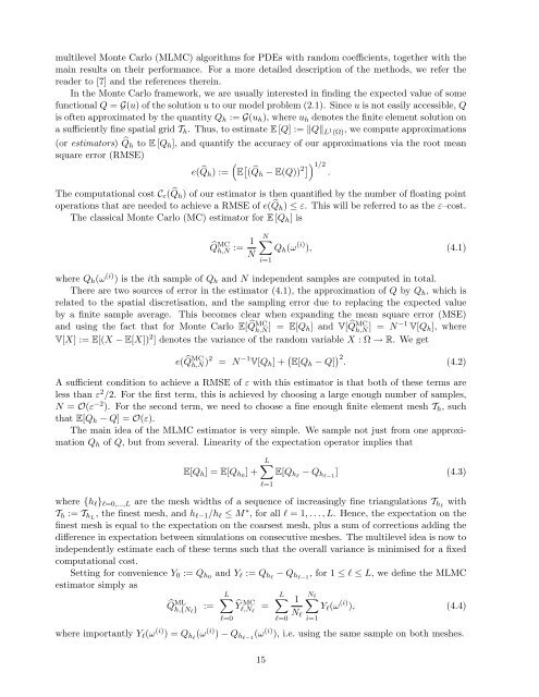
multilevel Monte Carlo (MLMC) algorithms for PDEs with random coefficients, together with themain results on their performance. For a more detailed description of the methods, we refer thereader to [7] and the references therein.In the Monte Carlo framework, we are usually interested in finding the expected value of somefunctional Q = G(u) of the solution u to our model problem (2.1). Since u is not easily accessible, Qis often approximated by the quantity Q h := G(u h ), where u h denotes the finite element solution ona sufficiently fine spatial grid T h . Thus, to estimate E [Q] := ‖Q‖ L 1 (Ω), we compute approximations(or estimators) ̂Q h to E [Q h ], and quantify the accuracy of our approximations via the root meansquare error (RMSE)e( ̂Q(h ) := E [ ( ̂Q h − E(Q)) 2]) 1/2.The computational cost C ε ( ̂Q h ) of our estimator is then quantified by the number of floating pointoperations that are needed to achieve a RMSE of e( ̂Q h ) ≤ ε. This will be referred to as the ε–cost.The classical Monte Carlo (MC) estimator for E [Q h ] iŝQ MCh,N := 1 NN∑Q h (ω (i) ), (4.1)i=1where Q h (ω (i) ) is the ith sample of Q h and N independent samples are computed in total.There are two sources of error in the estimator (4.1), the approximation of Q by Q h , which isrelated to the spatial discretisation, and the sampling error due to replacing the expected valueby a finite sample average. This becomes clear when expanding the mean square error (MSE)and using the fact that for Monte Carlo E[ ̂QMCh,N ] = E[Q h] and V[ ̂QMCh,N ] = N −1 V[Q h ], whereV[X] := E[(X − E[X]) 2 ] denotes the variance of the random variable X : Ω → R. We getMCe( ̂Q h,N )2 = N −1 V[Q h ] + ( E[Q h − Q] ) 2 . (4.2)A sufficient condition to achieve a RMSE of ε with this estimator is that both of these terms areless than ε 2 /2. For the first term, this is achieved by choosing a large enough number of samples,N = O(ε −2 ). For the second term, we need to choose a fine enough finite element mesh T h , suchthat E[Q h − Q] = O(ε).The main idea of the MLMC estimator is very simple. We sample not just from one approximationQ h of Q, but from several. Linearity of the expectation operator implies thatE[Q h ] = E[Q h0 ] +L∑E[Q hl − Q hl−1 ] (4.3)l=1where {h l } l=0,...,L are the mesh widths of a sequence of increasingly fine triangulations T hl withT h := T hL , the finest mesh, and h l−1 /h l ≤ M ∗ , for all l = 1, . . . , L. Hence, the expectation on thefinest mesh is equal to the expectation on the coarsest mesh, plus a sum of corrections adding thedifference in expectation between simulations on consecutive meshes. The multilevel idea is now toindependently estimate each of these terms such that the overall variance is minimised for a fixedcomputational cost.Setting for convenience Y 0 := Q h0 and Y l := Q hl − Q hl−1 , for 1 ≤ l ≤ L, we define the MLMCestimator simply aŝQ L MLh,{N l } := ∑L∑Ŷl,N MC 1 ∑N ll=Y l (ω (i) ), (4.4)l=0N ll=0 i=1where importantly Y l (ω (i) ) = Q hl (ω (i) ) − Q hl−1 (ω (i) ), i.e. using the same sample on both meshes.15
Since all the expectations E[Y l ] are estimated independently in (4.3), the variance of the MLMCestimator is ∑ LV[Y l ] and expanding as in (4.2) leads again tol=0 N −1lMLe( ̂Qh,{N l } )2[ ( ]:= E ̂QML h,{N l } − E[Q]) 2=L∑l=0N −1lV[Y l ] + ( E[Q h − Q] ) 2 . (4.5)As in the classical MC case before, we see that the MSE consists of two terms, the variance of theestimator and the error in mean between Q and Q h . Note that the second term is identical to thesecond term for the classical MC method in (4.2). A sufficient condition to achieve a RMSE of ε isagain to make both terms less than ε 2 /2. This is easier to achieve with the MLMC estimator, as• for sufficiently large h 0 , samples of Q h0 are much cheaper to obtain than samples of Q h ;• the variance Y l tends to 0 as h l → 0, meaning we need fewer samples on T hl , for l > 0.Let now C l denote the cost to obtain one sample of Q hl . Then we have the following results on theε–cost of the MLMC estimator (cf. [7, 16]).Theorem 4.1. Suppose that there are positive constants α, β, γ > 0 such that α≥ 1 2min(β, γ) andM1. |E[Q h − Q]| = O(h α )M2. V[Q hl − Q hl−1 ] = O(h β l )M2. C l = O(h −γl),Then, for any ε γ,⎨MLC ε ( ̂Qh,{N l } ) ε −2 (log ε) 2 , if β = γ,⎪ ⎩ε −2−(γ−β)/α , if β < γ.For the classical MC estimator we have C ε ( ̂QMCh ) = O(ε−2−γ/α ).We can now use the results from Section 3.2 to verify Assumptions M1–M2 in Theorem 4.1for some simple functionals G(u). More complicated functionals could then be tackled by dualityarguments in a similar way.Proposition 4.2. Let Q = G(u) := |u| q H 1 (D) , for some 1 ≤ q ded domain and that Assumptions A1–A4 hold, for some 0 < t < 1. Then AssumptionsM1–M2 in Theorem 4.1 hold for any α < t and β < 2t. For t = 1, we get α = 1 and β = 2.Proof. We only give the proof for t < 1. The proof for t = 1 is analogous. Let Q h := |u h | q H 1 (D) .Using the expansion a q − b q = (a − b) ∑ q−1j=0 aj b q−1−j , for a, b ∈ R and q ∈ N, we get{}|Q(ω) − Q h (ω)| |u(ω, ·) − u h (ω, ·)| H 1 (D) max |u(ω, ·)| q−1H 1 (D) , |u h(ω, ·)| q−1H 1 (D) , 1 , almost surely.This also holds for non-integer values of q > 1. Now, it follows from Lemma 2.1 and Theorem 3.9that, for any α < t,|Q(ω) − Q h (ω)| C 3.1(ω) C 3.8 (ω)a q−1min (ω) ‖f(ω, ·)‖ q H α−1 (D) hα , almost surely.16
Page 1 and 2: BICSBath Institute for Complex Syst
Page 3 and 4: only Hölder continuous with expone
Page 5 and 6: for almost all ω ∈ Ω. The diffe
Page 7 and 8: 2.4 Truncated Karhunen-Loève Expan
Page 9 and 10: 3.1 Regularity of the SolutionPropo
Page 11 and 12: Theorem 3.4. Let Assumptions A1-A3
Page 13 and 14: Corollary 3.10. Let Assumptions A1-
Page 15: 3.4 Truncated FieldsCombining the r
Page 19 and 20: Figure 1: Let d = 1 and σ 2 = 1 in
Page 21 and 22: Figure 4: Left: Number of samples N
Page 23 and 24: therefore we getA min ‖(R i h )
Page 25 and 26: ∥∂which means that2 ˜w∂x i
Page 27 and 28: Proof. Since supp(u 0 ) ⊂ D 0 , w
Page 29 and 30: We now extend A i to R d +. Since w

Bath Institute For Complex Systems - ENS de Cachan - Antenne de ...

Create successful ePaper yourself

Delete template?

Save as template?