Bath Institute For Complex Systems - ENS de Cachan - Antenne de ...

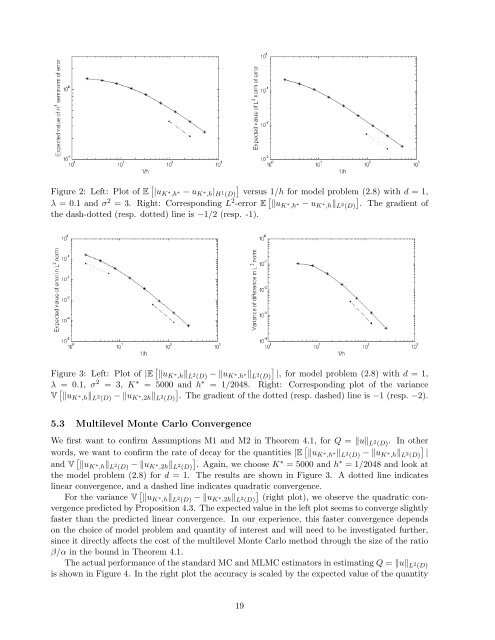
Figure 2: Left: Plot of E [ |u K ∗ ,h ∗ − u K ∗ ,h| H 1 (D)]versus 1/h for model problem (2.8) with d = 1,λ = 0.1 and σ 2 = 3. Right: Corresponding L 2 -error E [ ‖u K ∗ ,h ∗ − u K ∗ ,h‖ L 2 (D)]. The gradient ofthe dash-dotted (resp. dotted) line is −1/2 (resp. -1).Figure 3: Left: Plot of |E [ ‖u K ∗ ,h‖ L 2 (D) − ‖u K ∗ ,h ∗‖ L 2 (D)]|, for model problem (2.8) with d = 1,λ = 0.1, σ 2 = 3, K ∗ = 5000 and h ∗ = 1/2048. Right: Corresponding plot of the varianceV [ ‖u K ∗ ,h‖ L 2 (D) − ‖u K ∗ ,2h‖ L 2 (D)]. The gradient of the dotted (resp. dashed) line is −1 (resp. −2).5.3 Multilevel Monte Carlo ConvergenceWe first want to confirm Assumptions M1 and M2 in Theorem 4.1, for Q = ‖u‖ L 2 (D). In otherwords, we want to confirm the rate of decay for the quantities |E [ ‖u K ∗ ,h ∗‖ L 2 (D) − ‖u K ∗ ,h‖ L 2 (D)]|and V [ ‖u K ∗ ,h‖ L 2 (D) − ‖u K ∗ ,2h‖ L 2 (D)]. Again, we choose K ∗ = 5000 and h ∗ = 1/2048 and look atthe model problem (2.8) for d = 1. The results are shown in Figure 3. A dotted line indicateslinear convergence, and a dashed line indicates quadratic convergence.For the variance V [ ‖u K ∗ ,h‖ L 2 (D) − ‖u K ∗ ,2h‖ L 2 (D)](right plot), we observe the quadratic convergencepredicted by Proposition 4.3. The expected value in the left plot seems to converge slightlyfaster than the predicted linear convergence. In our experience, this faster convergence dependson the choice of model problem and quantity of interest and will need to be investigated further,since it directly affects the cost of the multilevel Monte Carlo method through the size of the ratioβ/α in the bound in Theorem 4.1.The actual performance of the standard MC and MLMC estimators in estimating Q = ‖u‖ L 2 (D)is shown in Figure 4. In the right plot the accuracy is scaled by the expected value of the quantity19