analysis of water injection into high-temperature mixture of ...

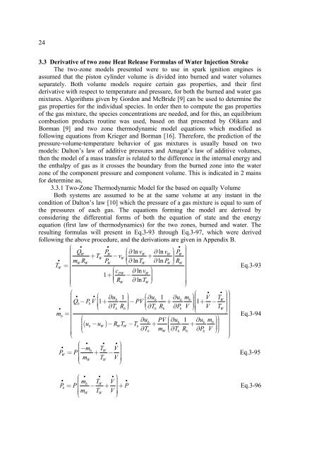
243.3 Derivative of two zone Heat Release Formulas of Water Injection StrokeThe two-zone models presented were to use in spark ignition engines isassumed that the piston cylinder volume is divided into burned and water volumesseparately. Both volume models require certain gas properties, and their firstderivative with respect to temperature and pressure, for both the burned and water gasmixtures. Algorithms given by Gordon and McBride [9] can be used to determine thegas properties for the individual species. In order then to compute the gas propertiesof the gas mixture, the species concentrations are needed, and for this, an equilibriumcombustion products routine was used, based on that presented by Olikara andBorman [9] and two zone thermodynamic model equations which modified asfollowing equations from Krieger and Borman [16]. Therefore, the prediction of thepressure-volume-temperature behavior of gas mixtures is usually based on twomodels: Dalton’s law of additive pressures and Amagat’s law of additive volumes,then the model of a mass transfer is related to the difference in the internal energy andthe enthalpy of gas as it crosses the boundary from the burned zone into the waterzone of the component pressure and component volume. This is indicated in 2 mainsfor determine as,3.3.1 Two-Zone Thermodynamic Model for the based on equally VolumeBoth systems are assumed to be at the same volume at any instant in thecondition of Dalton’s law [10] which the pressure of a gas mixture is equal to sum ofthe pressures of each gas. The equations forming the model are derived byconsidering the differential forms of both the equation of state and the energyequation (first law of thermodynamics) for the two zones, burned and water. Theresulting formulas will present in Eq.3-93 through Eq.3-97, which were derivedfollowing the above procedure, and the derivations are given in Appendix B.⎛• ••⎛ ln ln ⎞⎞Q WPW ∂ vW ∂ vW+ − +P •TWvWW⎜∂⎜ ln ∂ln⎟m ⎝= WRW PW TW PW ⎠RWTWEq.3-93⎛ ∂ ln ⎞1+ cPWvW−⎜⎜ ∂ ln⎝ R ⎟⎠ ⎜⎝WTW⎟⎠⎛• • ⎞• • ⎛ 1 ⎞ ⎛ 1 ⎞⎛ ⎞ ∂ub ⎜1 ∂ub ∂ub mb⎟⎜V T − + − + 1+ −QbPbV ⎜PVW⎟⎜⎟•⎝ ∂Tb Rb⎠ ⎝∂Tb Rb ∂Pb V ⎠⎜⎜V T⎝W ⎟m = b⎛ ∂ ⎛∂ Eq.3-941 ∂ ⎞⎞ub PV( − ) − − + ub ub mb+u buW RWTW T⎠⎟b⎜⎝∂ ⎜T ⎝⎜∂ ∂ ⎠⎟⎟⎠b mW Tb Rb Pb V⎜⎝⎟⎠⎛ • • • ⎞•−mbTWVPW= P + −Eq.3-95⎜ mW TW V⎜⎝⎟⎠⎛• • •• mbTWV•Pb= P − + + P⎜mWTWV⎟⎜⎝⎞ ⎟⎟⎠Eq.3-96