Sweating the Small Stuff: Does data cleaning and testing ... - Frontiers

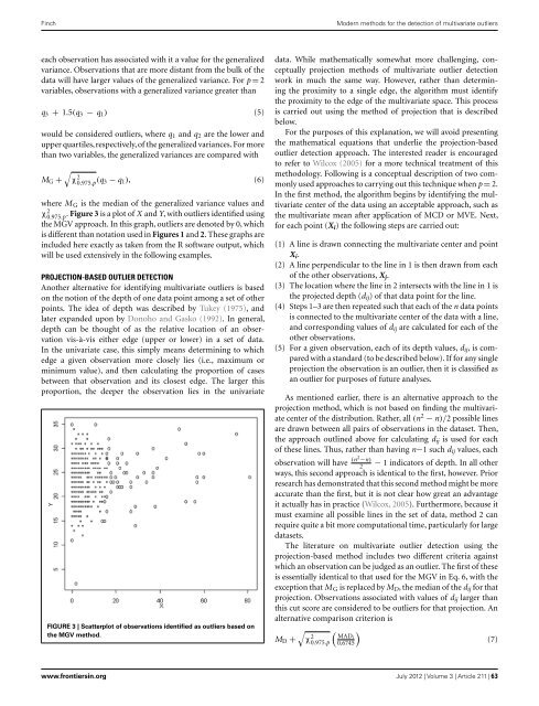
FinchModern methods for the detection of multivariate outlierseach observation has associated with it a value for the generalizedvariance. Observations that are more distant from the bulk of thedata will have larger values of the generalized variance. For p = 2variables, observations with a generalized variance greater thanq 3 + 1.5(q 3 − q 1 ) (5)would be considered outliers, where q 1 and q 2 are the lower andupper quartiles,respectively,of the generalized variances. For morethan two variables, the generalized variances are compared with√M G + χ 2 0.975.p (q 3 − q 1 ), (6)where M G is the median of the generalized variance values andχ 2 0.975.p . Figure 3 is a plot of X and Y, with outliers identified usingthe MGV approach. In this graph, outliers are denoted by 0, whichis different than notation used in Figures 1 and 2. These graphs areincluded here exactly as taken from the R software output, whichwill be used extensively in the following examples.PROJECTION-BASED OUTLIER DETECTIONAnother alternative for identifying multivariate outliers is basedon the notion of the depth of one data point among a set of otherpoints. The idea of depth was described by Tukey (1975), andlater expanded upon by Donoho and Gasko (1992). In general,depth can be thought of as the relative location of an observationvis-à-vis either edge (upper or lower) in a set of data.In the univariate case, this simply means determining to whichedge a given observation more closely lies (i.e., maximum orminimum value), and then calculating the proportion of casesbetween that observation and its closest edge. The larger thisproportion, the deeper the observation lies in the univariateFIGURE 3 | Scatterplot of observations identified as outliers based onthe MGV method.data. While mathematically somewhat more challenging, conceptuallyprojection methods of multivariate outlier detectionwork in much the same way. However, rather than determiningthe proximity to a single edge, the algorithm must identifythe proximity to the edge of the multivariate space. This processis carried out using the method of projection that is describedbelow.For the purposes of this explanation, we will avoid presentingthe mathematical equations that underlie the projection-basedoutlier detection approach. The interested reader is encouragedto refer to Wilcox (2005) for a more technical treatment of thismethodology. Following is a conceptual description of two commonlyused approaches to carrying out this technique when p = 2.In the first method, the algorithm begins by identifying the multivariatecenter of the data using an acceptable approach, such asthe multivariate mean after application of MCD or MVE. Next,for each point (X i ) the following steps are carried out:(1) A line is drawn connecting the multivariate center and pointX i .(2) A line perpendicular to the line in 1 is then drawn from eachof the other observations, X j .(3) The location where the line in 2 intersects with the line in 1 isthe projected depth (d ij ) of that data point for the line.(4) Steps 1–3 are then repeated such that each of the n data pointsis connected to the multivariate center of the data with a line,and corresponding values of d ij are calculated for each of theother observations.(5) For a given observation, each of its depth values, d ij , is comparedwith a standard (to be described below). If for any singleprojection the observation is an outlier, then it is classified asan outlier for purposes of future analyses.As mentioned earlier, there is an alternative approach to theprojection method, which is not based on finding the multivariatecenter of the distribution. Rather, all (n 2 − n)/2 possible linesare drawn between all pairs of observations in the dataset. Then,the approach outlined above for calculating d ij is used for eachof these lines. Thus, rather than having n−1 such d ij values, eachobservation will have (n2 −n)2− 1 indicators of depth. In all otherways, this second approach is identical to the first, however. Priorresearch has demonstrated that this second method might be moreaccurate than the first, but it is not clear how great an advantageit actually has in practice (Wilcox, 2005). Furthermore, because itmust examine all possible lines in the set of data, method 2 canrequire quite a bit more computational time, particularly for largedatasets.The literature on multivariate outlier detection using theprojection-based method includes two different criteria againstwhich an observation can be judged as an outlier. The first of theseis essentially identical to that used for the MGV in Eq. 6, with theexception that M G is replaced by M D , the median of the d ij for thatprojection. Observations associated with values of d ij larger thanthis cut score are considered to be outliers for that projection. Analternative comparison criterion is√ ( )M D + χ 2 MADi0.975.p 0.6745(7)www.frontiersin.org July 2012 | Volume 3 | Article 211 | 63