Sweating the Small Stuff: Does data cleaning and testing ... - Frontiers

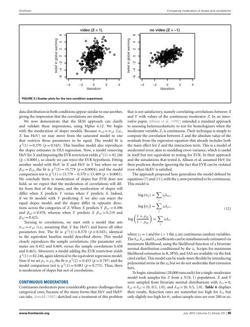
SmithsonComparing moderation of slopes and correlationsvideo (Z = 1)no video (Z = −1)belief in global warming−6 −4 −2 0 2 4 6belief in global warming−6 −4 −2 0 2 4 6−4 −2 0 2 4liberalism−4 −2 0 2 4liberalismFIGURE 3 | Scatter plots for the two-condition experiment.data distribution in both conditions appear similar to one another,giving the impression that the correlations are similar.We now demonstrate that the SEM approach can clarifyand validate these impressions, using Mplus 6.12. We beginwith the moderation of slopes models. Because σ x1 = σ x2 (i.e.,X has HoV) we may move from the saturated model to onethat restricts those parameters to be equal. The model fit isχ 2 (1) = 0.370 (p = 0.543). This baseline model also reproducesthe slopes estimates in OLS regression. Now, a model removingHoV for X and imposing the EVR restriction yields χ 2 (1) = 82.246(p < 0.0001), so clearly we can reject the EVR hypothesis. Fittinganother model with HoV in X and HeV in Y but where we setβ y1 = β y2 , the fit is χ 2 (2) = 15.779 (p = 0.0004), and the modelcomparison test is χ 2 (1) = 15.779 − 0.370 = 15.409 (p < 0.0001).We conclude there is moderation of slopes but EVR does nothold, so we expect that the moderation of correlations will differfrom that of the slopes, and the moderation of slopes willdiffer when X predicts Y versus when Y predicts X. Indeed,if we fit models with Y predicting X we also can reject theequal slopes model, and the slopes differ in opposite directionsacross the categories of Z. When X predicts Y β y1 = 0.496and β y2 = 0.978, whereas when Y predicts X β x1 = 0.219 andβ x2 = 0.423.Turning to correlations, we start with a model that setsσ x1 = σ x2 (i.e., assuming that X has HoV) and leaves all otherparameters free. The fit is χ 2 (1) = 0.370 (p = 0.543), identicalto the equivalent baseline model described above. This modelclosely reproduces the sample correlations (the parameter estimatesare 0.452 and 0.469, versus the sample correlations 0.458and 0.463). Moreover, a model adding the EVR restriction yieldsχ 2 (1) = 82.246, again identical to the equivalent regression model.Now if we set ρ 1 = ρ 2 , the fit is χ 2 (2) = 0.453 (p = 0.797) and themodel comparison test is χ 2 (1) = 0.083 (p = 0.773). Thus, thereis moderation of slopes but not of correlations.CONTINUOUS MODERATORSContinuous moderators pose considerably greater challenges thancategorical ones, because of the many forms that HeV and HeEVcan take. Arnold (1982) sketched out a treatment of this problemthat is not satisfactory, namely correlating correlations between Xand Y with values of the continuous moderator Z. In an innovativepaper, Allison et al. (1992) extended a standard approachto assessing heteroscedasticity to test for homologizers when themoderator variable, Z, is continuous. Their technique is simply tocompute the correlation between Z and the absolute value of theresiduals from the regression equation that already includes boththe main effect for Z and the interaction term. This is a model ofmoderated error, akin to modeling error-variance, which is usefulin itself but not equivalent to testing for EVR. In their approachand the simulations that tested it, Allison et al. assumed HeV fortheir predictor, thereby ignoring the fact that EVR can be violatedeven when HeEV is satisfied.The approach proposed here generalizes the model defined byequations (7) and (11),with the z i now permitted to be continuous.This model islog (σ x ) = ∑ z i δ xi ,ilog ( ) ∑σ y = z i δ yi ,( ) 1 + ρxylog= ∑ 1 − ρ xyiiz i δ ri(12)where z 1 = 1 and for i > 1 the z i are continuous random variables.The δ xi ,δ yi , and δ ri coefficients can be simultaneously estimated viamaximum likelihood, using the likelihood function of a bivariatenormal distribution conditioned by the z i . Scripts for maximumlikelihood estimation in R, SPSS, and SAS are available via the linkcited earlier. This model can be made more flexible by introducingpolynomial terms in the z i , but we do not undertake that extensionhere.To begin, simulations (20,000 runs each) for a single-moderatormodel took samples for Z from a N (0, 1) population. X and Ywere sampled from bivariate normal distributions with δ r1 = 0,δ x1 = δ y1 = {0, 0.5, 1.0}, and δ r0 = {0, 0.5, 1.0}. Table 6 displaystheir results. Rejection rates are somewhat too high for δ r1 butonly slightly too high for θ 1 unless sample sizes are over 200 or so.www.frontiersin.org July 2012 | Volume 3 | Article 231 | 98