Seismic 2D Reflection Processing and Interpretation of ... - Posiva

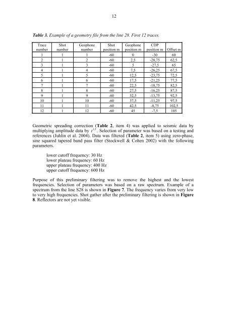
12Table 3. Example of a geometry file from the line 28. First 12 traces.TracenumberShotnumberGeophonenumberShotposition mGeophoneposition mCDPposition mOffset m1 1 1 -60 0 -30 602 1 2 -60 2,5 -28,75 62,53 1 3 -60 5 -27,5 654 1 4 -60 7,5 -26,25 67,55 1 5 -60 12,5 -23,75 72,56 1 6 -60 17,5 -21,25 77,57 1 7 -60 22,5 -18,75 82,58 1 8 -60 27,5 -16,25 87,59 1 9 -60 32,5 -13,75 92,510 1 10 -60 37,5 -11,25 97,511 1 11 -60 42,5 -8,75 102,512 1 12 -60 45 -7,5 105Geometric spreading correction (Table 2, item 4) was applied to seismic data by1,5multiplying amplitude data by t . Selection of parameter was based on a testing andreferences (Juhlin et al. 2004). Data was filtered (Table 2, item 5) using zero-phase,sine squared tapered band pass filter (Stockwell & Cohen 2002) with the followingparameters.lower cutoff frequency: 30 Hzlower plateau frequency: 60 Hzupper plateau frequency: 400 Hzupper cutoff frequency: 600 HzPurpose of this preliminary filtering was to remove the highest and the lowestfrequencies. Selection of parameters was based on a raw spectrum. Example of aspectrum from the line S28 is shown in Figure 7. The frequency varies from very lowto very high frequencies. Shot gather after the preliminary filtering is shown in Figure8. Reflectors are not yet visible.