Satellite detection of hazardous volcanic clouds and ... - Savaa - NILU

More documents

Recommendations

Info

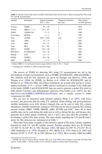
Nat HazardsTable 3 Details of past and current satellite instruments that can be used to detect and quantify SO 2 usingUV and IR measurementsSatellite Instrument Spatial resolution(km 9 km)Temporal resolution(per day)Time periodcovered (present)Various TOMS 50 9 50 1 1979NOAA HIRS-2, -3, -4 10 9 10 a 2 1979GOES VISSR/VAS 5 9 5 24 1980Terra/Aqua MODIS 1 9 1 4 b 1999Terra ASTER 0.09 9 0.09 1/16 1999Aqua AIRS 14 9 14 2 2002Aura OMI 24 9 13 1 2004Aura MLS 30 9 150 1 2004ERS-2 GOME 320 9 40 1 1995ENVISAT SCIAMACHY 60 9 30 1 2002MetOp IASI 12 9 12 2 2007MetOp GOME-2 80 9 40 2 2007MSG SEVIRI 3 9 3 96 2006a Earlier HIRS (1–3) instruments had a larger field of view of 18 9 18 km 2b Assuming two satellites in orbit at any given timeThe success of TOMS for detecting SO 2 using UV measurements has led to thedevelopment of improved instruments such as GOME, SCIAMACHY, OMI and GOME-2.The methods used for SO 2 detection are given by Eisinger and Burrows (1998) andThomas et al. (2004) for GOME, by Richter et al. (2006) for SCIAMACHY and byKrotkov et al. (2006) for OMI. All of these instruments are in polar orbit and have, at best,spatial resolutions of 14 9 24 km 2 (OMI) and are restricted to coverage of the sunlit partof the Earth. GOME-2 and SCIAMACHY data are used to generate a global SO 2 alert forboth natural (volcanic) and anthropogenic emissions (Van Geffen et al. (2007), see alsohttp://www.oma.be/BIRA-IASB/Molecules/SO2nrt/) and a similar system is underconstruction for OMI.SO 2 can also be measured using infrared radiation (Prata et al. 2003), with loweraccuracy and precision than by using UV radiation. Polar-orbiting and geosynchronoussatellite instruments exist with infrared channels that can be used to infer SO 2 columnabundances. Satellite instruments starting in 1979 that can be used to measure SO 2 columnamount include: HIRS, VISSR, MODIS, AIRS, SEVIRI and IASI. 2 Since all of thesesatellite data can be used during the night just as well as during the day, and because theygenerally have better spatial resolutions (up to 1 km 2 ), they also offer the possibility ofdeveloping a global SO 2 alert system. The main details regarding the UV and IR instrumentsfor SO 2 detection are summarized in Table 3.There have been many examples of the extensive spread of SO 2 from volcanic eruptionsdetected by both UV and IR satellite sensors. Notable amongst these are El Chichon(17.360° N, 92.228° W) in 1982 (Krueger 1983), Mt Spurr (61.299° N, 152.251° W) in1989 (Schneider et al. 1995), Pinatubo in 1991 (Bluth et al. 1993; Prata et al. 2003) andHudson (45.90° S, 72.97° W) in 1991 (Barton et al. 1992). More recently, OMI and AIRS2 ASTER can also be used to detect volcanic SO 2 (e.g. Urai 2004), but its long re-visit time (16 days) andnarrow swath width (*60 km) make it less useful for global aviation threat monitoring.123
Nat Hazardsmeasurements have tracked clouds of SO 2 generated by eruptions from Soufriere Hills,Montserat (16.72° N, 62.18° W) (Carn et al. 2007; Prata et al. 2007) and Jebel at Tair,Yemen (Eckhardt et al. 2008). These SO 2 clouds could be tracked for several weeks asthey travelled with the prevailing winds at heights greater than 15 km. At these heights theSO 2 clouds were above commercial jet aircraft traffic and posed little threat to aviation, butthis may not always be the case. The ability to track and forecast the movement ofhazardous clouds using satellite-based SO 2 measurements is of great value and as indicatedearlier, global alert systems have been developed to provide aviation warnings using thesedata.5 The global threat to aviation from volcanic eruption cloudsVolcanic clouds move with the prevailing winds at the height of injection. At the onset ofan eruption, it is likely that ash and gases are spread throughout the vertical column up tothe maximum height reached by the cloud, which depends on the energetics of the eruptionwith some dependency on environmental conditions. During the first few hours of eruption,the vicinity in the neighbourhood of the volcano poses the greatest threat to aviation.Usually precursor information about the activity of the volcano is available and aviation isalerted well before an eruption occurs. Following a significant eruption, the ash and gasescan be transported over great distances, but are usually confined to a much smaller verticalrange of 1–2 km. Dispersion modelling of the movement of the cloud then dependscritically on knowledge of the location of the cloud in the vertical, and less on the windfields, as these are generally known more accurately. Current practice is to guess the heightof the cloud based upon trial-and-error fits between observations of the clouds and modelruns. VAACs use this information cautiously, together with other sources of information.They will advise that airspace is affected from the ground up to the suspected maximumheight of the volcanic cloud, and express this in aviation terminology using flight levels,e.g. FL 350 means a pressure altitude of 35,000 ft or 10,700 m. Air traffic should thendivert around a rather large spatial region which covers the horizontal location of the cloudand the vertical region from the ground up to FL X, where X is the designated flightlevel affected. While this strategy is risk averse, it can be a financial burden and perhapsunnecessary for the operator. This is because the volcanic cloud will, in most cases, beconfined in the vertical to a layer of 1–2 km thickness and may not contain ash. The residencetime of fine ash in the upper troposphere is of the order of several hours to a fewdays, and in a dispersed state the ash may not be a hazard to aircraft, although some casestudies seem to indicate even undetected, very low concentration ash clouds may still posea threat (Pieri et al. 2002; Tupper et al. 2004). Given the range of uncertainties present inpredicting volcanic eruption activity, in knowledge of the injection height profile of aneruption and in establishing the minimum ash concentration level that is still dangerous toaviation, only fairly general indications of vulnerability can be established.The mid- and upper-troposphere (MUT) wind circulation patterns are fundamental toestablishing the hazard posed to commercial inter-continental aviation from dispersingvolcanic clouds. In the MUT, zonal winds are stronger than meridional winds and consequentlyvolcanic clouds tend to travel rapidly in the zonal direction. The long-term meanzonal wind fields at 250 hPa (10 km) are shown in Fig. 4 for the months of January(Fig. 4a) and July (Fig. 4b). Most notable in these plots are the strong zonal jets at roughly30° N in January and 30° S in July. Zonal winds are generally quite weak ±10° latitudeeither side of the equator, but there is a noticeable seasonal dependence, with easterlies123
Page 1 and 2: Nat HazardsDOI 10.1007/s11069-008-9
Page 3 and 4: Nat HazardsThe article is organized
Page 5 and 6: Nat Hazardscloud. Figure 1a-h shows
Page 7 and 8: Nat HazardsFig. 2 An ash ‘‘risk
Page 9: Nat Hazardsinferred later. Once a s
Page 13 and 14: Nat Hazardsdominating at latitudes
Page 15 and 16: Nat HazardsFig. 6 Latitude-height c
Page 17 and 18: Nat HazardsHolocene and historicall
Page 19 and 20: Nat Hazardscloud encounters. The in
Page 21 and 22: Nat HazardsHolasek RE, Woods AW, Se

Satellite detection of hazardous volcanic clouds and ... - Savaa - NILU

You also want an ePaper? Increase the reach of your titles

Delete template?

Save as template?