DBI Analysis of Open String Bound States on Non-compact D-branes

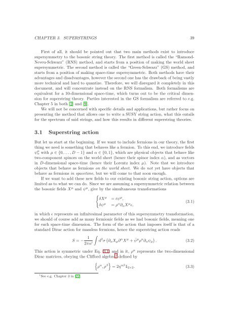
CHAPTER 3. SUPERSTRINGS 39First <strong>of</strong> all, it should be pointed out that two main methods exist to introducesupersymmetry to the bosonic string theory. The first method is called the “Ramond-Neveu-Schwarz” (RNS) method, and starts from a position <strong>of</strong> making the world sheetsupersymmetric. The second method is called the “Green-Schwarz” (GS) method, andstarts from a position <strong>of</strong> making space-time supersymmetric. Both methods have theiradvantages and disadvantages, however the second one has the drawback <strong>of</strong> being vastlymore technical and hard to quantize. Therefore, we will disregard it completely in thisdocument, and will concentrate instead on the RNS formalism. Both formalisms areequivalent for a 10-dimensional space-time, which turns out to be the critical dimensionfor superstring theory. Parties interested in the GS formalism are referred to e.g.Chapter 5 in both [2] and [9].We will not be concerned with specific details and applications, but rather focus onpresenting the method that allows one to write a SUSY string action, what this entailsfor the spectrum <strong>of</strong> said strings, and how this results in different superstring theories.3.1 Superstring actionBut let us start at the beginning. If we want to include fermions in our theory, the firstthing we need is something that behaves like a fermion. To this end, we introduce fieldsψ α µ with µ ∈ {0, . . .,D − 1} and α ∈ {0, 1}, which are physical objects that behave liketwo-component spinors on the world sheet (hence their spinor index α), and as vectorsin D-dimensional space-time (hence their Lorentz index µ). Note that we introduceobjects that behave as fermions on the world sheet. We do not yet have objects thatbehave as fermions in spacetime, but we will come to that soon enough.If we want to add these new fields to our existing bosonic string action, options arelimited as to what we can do. Since we are assuming a supersymmetric relation betweenthe bosonic fields X µ and ψ µ , give by the simultaneous transformations{δX µ = ¯ǫψ µ ,δψ µ = ρ α ∂ α X µ (3.1)ǫ,in which ǫ represents an infinitesimal parameter <strong>of</strong> this supersymmetry transformation,we should <strong>of</strong> course add as many fermionic fields as we had bosonic fields, meaning onefor each space-time dimension. The form <strong>of</strong> the action that imposes itself is that <strong>of</strong> astandard Dirac action for massless fermions, hence the superstring action readsS = − 1 ∫2πα ′ d 2 σ ( ∂ α X µ ∂ α X µ + ¯ψ µ ρ α )∂ α ψ µ . (3.2)This action is symmetric under Eq. 3.1, and in it, ρ α represents the two-dimensionalDirac matrices, obeying the Clifford algebra 1 defined by{ρ α , ρ β} = 2η αβ½2×2. (3.3)1 See e.g. Chapter 3 in [22].