Fundamentals of Matrix Algebra, 2011a

Chapter 2
Matrix Arithmec
2.3 Visualizing Matrix Arithmec in 2D
AS YOU READ ...
. . .
1. T/F: Two vectors with the same length and direcon are equal even if they start
from different places.
2. One can visualize vector addion using what law?
3. T/F: Mulplying a vector by 2 doubles its length.
4. What do mathemacians do?
5. T/F: Mulplying a vector by a matrix always changes its length and direcon.
When we first learned about adding numbers together, it was useful to picture a
number line: 2 + 3 = 5 could be pictured by starng at 0, going out 2 ck marks, then
another 3, and then realizing that we moved 5 ck marks from 0. Similar visualizaons
helped us understand what 2 − 3 meant and what 2 × 3 meant.
We now invesgate a way to picture matrix arithmec – in parcular, operaons
involving column vectors. This not only will help us beer understand the arithmec
operaons, it will open the door to a great wealth of interesng study. Visualizing
matrix arithmec has a wide variety of applicaons, the most common being computer
graphics. While we oen think of these graphics in terms of video games, there are
numerous other important applicaons. For example, chemists and biologists oen
use computer models to “visualize” complex molecules to “see” how they interact with
other molecules.
We will start with vectors in two dimensions (2D) – that is, vectors with only two
entries. We assume the reader is familiar with the Cartesian plane, that is, plong
points and graphing funcons on “the x–y plane.” We graph vectors in a manner very
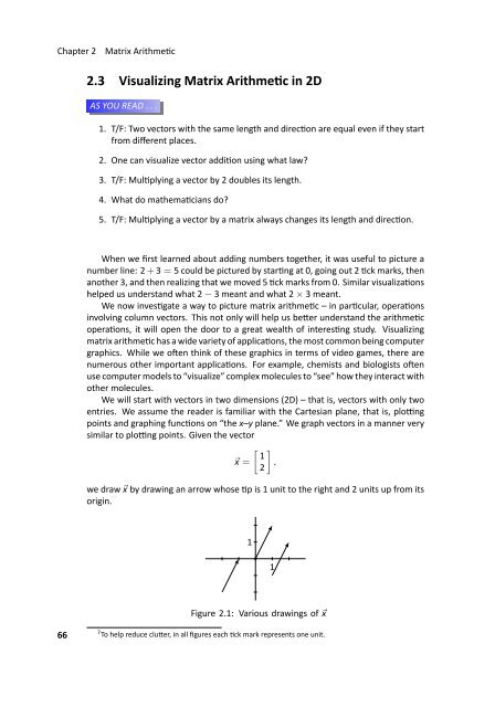
similar to plong points. Given the vector
[ ] 1
⃗x = ,
2
we draw ⃗x by drawing an arrow whose p is 1 unit to the right and 2 units up from its
origin. 7 .
1
.
1
.
Figure 2.1: Various drawings of ⃗x
66
7 To help reduce cluer, in all figures each ck mark represents one unit.