channel - Advances in Electronics and Telecommunications

60 ADVANCES IN ELECTRONICS AND TELECOMMUNICATIONS, VOL. 1, NO. 1, APRIL 2010
denotes the L × L identity matrix; diag{.} denotes a diagonal
matrix; ℜ{·} denotes the real part of {·}.
II. SIGNAL MODEL
We consider a synchronous CDMA system with K active
user sharing the same propagation channel and the signal
transmitted by each user experiences time-varying Rayleigh
fading over the observed frame of M symbols. The complex
baseband representation of the received signal, therefore, can
be expressed as
z(m) = RB(m)a(m) + n(m), m = 0, 1, · · · , M − 1 (1)
where z(m) = [z1(m), z2(m) · · · , zK(m)] T denote the complex
vector whose components represent K received signals
of the K respective users. The K × K diagonal matrix
B(m) is given by B(m) = diag {b1(m), b2(m) · · · , bK(m)}
, and bk ∈ {−1, +1}, denoting the binary symbols transmitted
by user k during the mth signaling interval. The
vector a = [a1(0), · · · , a1(M − 1), · · · , aK(0), · · · , aK(M −
1)] T represents the time-varying frequency-nonselective channel
whose components are modeled as complex circularly
symmetric Gaussian random variables and a(m) =
[a1(m), a2(m) · · · , aK(m)] T . The K × K matrix R of the
form
⎡
⎤
R �
⎢
⎣
1
.
· · ·
. ..
ρ1k
.
ρk1 · · · 1
with ρjk being the crosscorrelations between the signature
waveforms of user j and k.
While the wireless channel is time-varying frequencynonselective
at the receiver, then it is assumed to be modeled
according to a piece-wise constant channel. That is,
the channel is assumed to be constant during L consecutive
symbols. L is the parameter which may depend on the velocity
or the doppler frequency. Thus, the number of channel
coefficients to be estimated in an observation frame of M
symbols (M >> L) is reduced and the quality of the channel
estimation algorithm is improved. Following the piece-wise
constant channel model, Eq.(1) can be replaced by
z(m) = RB(m)a(⌊ m
⌋ + 1) + n(m), m = 0, 1, · · · , M − 1
L
(2)
where ⌊x⌋ denotes the integer which is less than or equal to x.
Let q � ⌊ m
L ⌋+1 then a(q) � [a1(q), a2(q), · · · , aK(q)] T , q =
1, 2, · · · , Ξ. ak � [ak(1), ak(2), · · · , ak(Ξ)] T is the reduced
vector of the channel coefficients and the integer Ξ is such that
LΞ = M. Finally, n(m) in (2) is a K−dimensional zero-mean
Gaussian random vector with covariance matrix N0R.
In general, the time variation of the channel coefficients can
be modeled using an autoregressive(AR)model of order n. For
first-order case, the channel coefficients of each user can be
expressed as
ak(q)=γkak(q − 1)+ǫk(q), k = 1,2,· · · ,K; q =1, 2, · · · , Ξ
(3)
where γk is the time correlation coefficients and ǫk(q) is the
additive white Gaussian noise (AWGN) with zero mean and
⎥
⎦
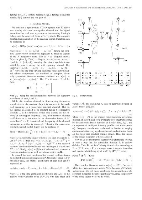
Fig. 1. System Model
variance σ 2 k . The parameter γk can be determined based on
Jakes’ model [16], [18]
rk(q − q ′ ) = σ 2 kJ0(2πfd(q − q)), for q, q ′ = 1, 2, ..., Ξ.
(4)
where rk(q − q ′ ) is the channel time-frequency covariance
function of the kth user for a Doppler power spectrum defined
by the zero-order Bessel function of the first kind, J0(.), and
an exponential multipath intensity profile with mean power
σ 2 k
. Computer simulations performed in Section 4, employ
continuously time-varying channel model, and estimated based
on the piece-wise constant channel model. Thus, the impact
of the model mismatch will be captured.
Now let us assume that the signature waveforms are selected
in such a way that the correlation function R is positive
definite. Then R can be Cholesky factorization according to
R = F T F, where F is a unique lower triangular invertible
real matrix. Multiplying z(m) in (2) by (F T ) −1 yields
y(m) � (F T ) −1 z(m) (5)
= FB(m)a(⌊ m
⌋ + 1) + w(m), m = 0, 1, · · · , M −1.
L
The complex Gaussian vector w(m) = (F T ) −1 n(m) is
white, i.e., has covariance matrix N0IK because of Cholesky
factorization. We will adopt employing this description of observation
model for the subsequent analysis, since the property
of the noise vector w(m) to be white.