ERCOFTAC Bulletin - Centre Acoustique

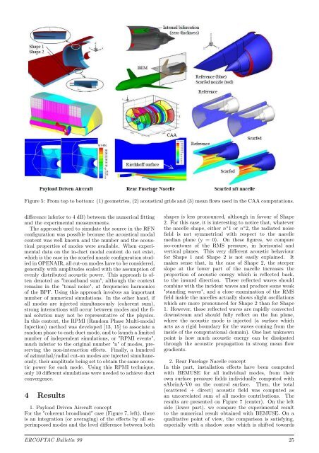
Figure 5: From top to bottom: (1) geometries, (2) acoustical grids and (3) mean flows used in the CAA computations.
difference inferior to 4 dB) between the numerical fitting
and the experimental measurements.
The approach used to simulate the source in the RFN
configuration was possible because the acoustical modal
content was well known and the number and the acoustical
properties of modes were available. When experimental
data on the in-duct modal content do not exist,
which is the case in the scarfed nozzle configuration studied
in OPENAIR, all cut-on modes have to be considered,
generally with amplitudes scaled with the assumption of
evenly distributed acoustic power. This approach is often
denoted as "broadband sum", although the context
remains in the "tonal noise", at frequencies harmonics
of the BPF. Using this approach involves an important
number of numerical simulations. In the other hand, if
all modes are injected simultaneously (coherent sum),
strong interactions will occur between modes and the final
solution may not be representative of the physics.
In this context, the RPMI (Random Phase Multi-modal
Injection) method was developed [13, 15] to associate a
random phase to each duct mode, and to launch a limited
number of independent simulations, or "RPMI events",
much inferior to the original number "n" of modes, preserving
the non-interaction effects. Finally, a hundred
of azimuthal/radial cut-on modes are injected simultaneously,
their amplitude being set to obtain the same acoustic
power for each mode. Using this RPMI technique,
only 10 different simulations were needed to achieve duct
convergence.
4 Results
1. Payload Driven Aircraft concept
For the "coherent broadband" case (Figure 7, left), there
is an integration (or averaging) of the effects by all superimposed
modes and the level difference between both
shapes is less pronounced, although in favour of Shape
2. For this case, it is interesting to notice that, whatever
the nacelle shape, either n ◦ 1 or n ◦ 2, the radiated noise
field is not symmetrical with respect to the nacelle
median plane (y = 0). On these figures, we compare
iso-contours of the RMS pressure, in horizontal and
vertical planes. This very different acoustic behaviour
for Shape 1 and Shape 2 is not easily explained. It
makes sense that, in the case of Shape 2, the steeper
slope at the lower part of the nacelle increases the
proportion of acoustic energy which is reflected back,
to the inward direction. These reflected waves should
combine with the incident waves and produce some weak
"standing waves", and a close examination of the RMS
field inside the nacelles actually shows slight oscillations
which are more pronounced for Shape 2 than for Shape
1. However, those reflected waves are rapidly convected
downstream and should fully reflect on the fan plane,
where the acoustic mode is injected (a surface which
acts as a rigid boundary for the waves coming from the
inside of the computational domain). One last unknown
point is how much acoustic energy can be dissipated
through the acoustic propagation in strong mean flow
gradients.
2. Rear Fuselage Nacelle concept
In this part, installation effects have been computed
with BEMUSE for all individual modes, from their
own surface pressure fields individually computed with
sAbrinA-V0 on the control surface. Then, the total
(scattered + direct) acoustic field was computed as
an uncorrelated sum of all modes contributions. The
results are presented on Figure 7 (center). On the left
side (lower part), we compare the experimental result
to the numerical result obtained with BEMUSE. On a
qualitative point of view, the comparison is satisfying,
especially with a shadow zone which is shifted towards
ERCOFTAC Bulletin 90 25