ERCOFTAC Bulletin - Centre Acoustique

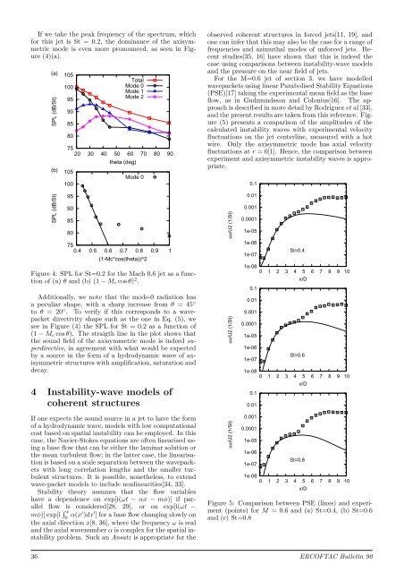
If we take the peak frequency of the spectrum, which
for this jet is St = 0.2, the dominance of the axisymmetric
mode is even more pronounced, as seen in Figure
(4)(a).
(a)
SPL (dB/St)
(b)
SPL (dB/St)
105
100
95
90
85
80
Total
Mode 0
Mode 1
Mode 2
75
20 30 40 50 60 70 80 90
105
100
95
90
85
80
theta (deg)
Mode 0
75
0.4 0.5 0.6 0.7 0.8 0.9 1
(1-Mc*cos(theta))^2
Figure 4: SPL for St=0.2 for the Mach 0.6 jet as a function
of (a) θ and (b) (1 − Mc cos θ) 2 .
Additionally, we note that the mode-0 radiation has
a peculiar shape, with a sharp increase from θ = 45 ◦
to θ = 20 ◦ . To verify if this corresponds to a wavepacket
directivity shape such as the one in Eq. (5), we
see in Figure (4) the SPL for St = 0.2 as a function of
(1 − Mc cos θ). The straigth line in the plot shows that
the sound field of the axisymmetric mode is indeed superdirective,
in agreement with what would be expected
by a source in the form of a hydrodynamic wave of axisymmetric
structures with amplification, saturation and
decay.
4 Instability-wave models of
coherent structures
If one expects the sound source in a jet to have the form
of a hydrodynamic wave, models with low computational
cost based on spatial instability can be employed. In this
case, the Navier-Stokes equations are often linearised using
a base flow that can be either the laminar solution or
the mean turbulent flow; in the latter case, the linearisation
is based on a scale separation between the wavepackets
with long correlation lengths and the smaller turbulent
structures. It is possible, nonetheless, to extend
wave-packet models to include nonlinearities[34, 33].
Stability theory assumes that the flow variables
have a dependence on exp[i(ωt − αx − mφ)] if parallel
flow is considered[28, 29], or on exp[i(ωt −
mφ)] exp[i x
0 α(x′ )dx ′ ] for a base flow changing slowly on
the axial direction x[8, 36], where the frequency ω is real
and the axial wavenumber α is complex for the spatial instability
problem. Such an Ansatz is appropriate for the
observed coherent structures in forced jets[11, 19], and
one can infer that this may also be the case for a range of
frequencies and azimuthal modes of unforced jets. Recent
studies[35, 16] have shown that this is indeed the
case using comparisons between instability-wave models
and the pressure on the near field of jets.
For the M=0.6 jet of section 3, we have modelled
wavepackets using linear Parabolised Stability Equations
(PSE)[17] taking the experimental mean field as the base
flow, as in Gudmundsson and Colonius[16]. The approach
is described in more detail by Rodriguez et al.[33],
and the present results are taken from this reference. Figure
(5) presents a comparison of the amplitudes of the
calculated instability waves with experimental velocity
fluctuations on the jet centerline, measured with a hot
wire. Only the axisymmetric mode has axial velocity
fluctuations at r = 0[1]. Hence, the comparison between
experiment and axisymmetric instability waves is appropriate.
uu/U2 (1/St)
uu/U2 (1/St)
uu/U2 (1/St)
0.1
0.01
0.001
0.0001
1e-05
1e-06
1e-07
St=0.4
1e-08
0 1 2 3 4 5 6 7 8 9 10
0.1
0.01
0.001
0.0001
1e-05
1e-06
1e-07
x/D
St=0.6
1e-08
0 1 2 3 4 5 6 7 8 9 10
0.1
0.01
0.001
0.0001
1e-05
1e-06
1e-07
x/D
St=0.8
1e-08
0 1 2 3 4 5 6 7 8 9 10
Figure 5: Comparison between PSE (lines) and experiment
(points) for M = 0.6 and (a) St=0.4, (b) St=0.6
and (c) St=0.8
36 ERCOFTAC Bulletin 90
x/D