ERCOFTAC Bulletin - Centre Acoustique

2.8 Filtering
The acoustic sources are usually given with a fine spatial
resolution on the grid of the flow simulation, while
the acoustic propagation allows a coarser grid. This can
cause aliasing effects, which lead to serious stability problems
in the acoustic simulation. Spatial filtering is a suitable
method to avoid this problem. In the presented calculation
a modal filter, as presented by Hesthaven [11],
was used. The basic idea is to eliminate the small scale
disturbances which can not be accurately resolved on the
coarser grid, by reducing the influence of the high order
modes:
u filtered
i = αi ui ∀ i = 1 . . . nDegF r (10)
The filter coefficients depend on the space order to which
the degrees of freedom i are related (see Table (1)). It
iDegF r 1 2 ... 3 4 ... 6 7 ... 10
αi 1.0000 0.9995 0.8688 0.0272
Table 1: Coefficients of modal filter for p = 3, nDegF r =
10
has to be made sure that the coefficient for the first degree
of freedom, which is the cell mean value, is equal
to one to ensure the conservation property of the filter.
For the presented calculations the filter was applied to
k u(tn) after each Taylor-DG step.
∂
∂t
3 The hybrid grid scheme -
PIANO+
As stated before, unstructured grids are very suitable
for simulations in complex shaped domains due to their
straightforward mesh generation. However, in the far
field the generation of structured grids is comparably
easy. Hence, it is favourable to benefit from the advantages
of structured solvers in terms of memory demand,
grid handling effort and visualization. This led to the
idea of coupling schemes for those different grid types.
These were the presented solver NoisSol and the finitedifference
(FD) solver PIANO (Perturbation Investigation
of Aerodynamic Noise [10]).
For the hybrid computation the computational domain
is splitted such, that both programs work on nonoverlapping
grids with straight coupling interfaces. The
information of the coupling partner are included using
ghost cells (DG) or ghost points (FD). There the continuity
of the primitive variables is enforced, which proved
to be the best way to prevent artificial reflections at the
interface. The data exchange is done by an extension of
the MPI infrastructure, that was already implemented
in both solvers.
The main focus in this coupling framework was on the
automatization of the coupling process to make it applicable
for industrial applications. For detailed information
about the coupled scheme see [8].
4 Application to airfoil noise - the
NASA 30P30N test case
One topic that is of great interest for computational
aeroacoustic applications in aerospace sciences is the
noise generation of an airfoil in high-lift configuration,
i.e., with deployed slat and flap.
This application is also a demanding test case for
acoustic simulation programs, since it combines a very
inhomogeneous flow, a complex geometry and many different
noise generation mechanisms. In this application
a three part airfoil is examined, which was described
by Lockard and Choudhari in 2009 [4]. The calculation
presented here bases on a RANS computation for an
unswept wing with an angle of attack of 4 ◦ , a Mach
number of 0.17 and a Reynolds number of 1.7e6. Based
on this flow field sound sources in 2D were calculated
by Roland Ewert of the IAS at the German Aerospace
Center (DLR) applying their Fast Random Particle
Mesh (FRPM) method [6]. The source calculation was
limited to a rectangular region around the slat trailing
edge (see Figure (1)).
The mean flow values have also been taken from the
RANS calculation.
The acoustic simulations were performed with the
Acoustic Perturbation Equations (APE), type 4 , see
Ewert and Schröder [7]. The space and time order
of the scheme were set to 4, the time step became
3.45e-5 in both cases. For the uncoupled simulation a
Figure 1: Setup NASA 30P30N (Arrow points to center
of microphone circle.)
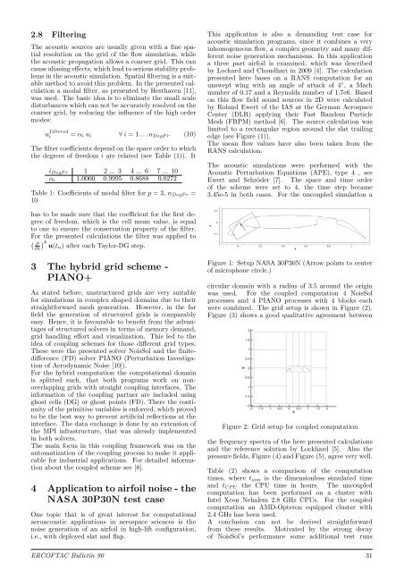
circular domain with a radius of 3.5 around the origin
was used. For the coupled computation 4 NoisSol
processes and 4 PIANO processes with 4 blocks each
were combined. The grid setup is shown in Figure (2).
Figure (3) shows a good qualitative agreement between
Figure 2: Grid setup for coupled computation
the frequency spectra of the here presented calculations
and the reference solution by Lockhard [5]. Also the
pressure fields, Figure (4) and Figure (5), agree very well.
Table (2) shows a comparison of the computation
times, where tsim is the dimensionless simulated time
and tCP U the CPU time in hours. The uncoupled
computation has been performed on a cluster with
Intel Xeon Nehalem 2.8 GHz CPUs. For the coupled
computation an AMD-Opteron equipped cluster with
2.4 GHz has been used.
A conclusion can not be derived straightforward
from these results. Motivated by the strong decay
of NoisSol’s performance some additional test runs
ERCOFTAC Bulletin 90 31