ERCOFTAC Bulletin - Centre Acoustique

The results of Figure (5) show a remarkable agreement
between the PSE results and the experiment up
to x/D ≈ 5, which is close to the end of the potential
core. It should be noted that since these are linear instability
waves, the PSE solution has a free amplitude. In
Figure (5) the amplitude was matched with the velocity
fluctuations at x = 2D.
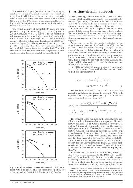
The sound radiation of the instability wave was computed
with Eq. (3), with T11(z, r, m = 0, ω) given as
ρ0U(z, r)u(z, r, m = 0, ω) , where U is the experimental
mean axial velocity and u(z, r, m = 0, ω) is given by
the PSE solution for the axisymmetric mode at each frequency.
Results, taken from Rodriguez et al.[33], are
shown in Figure (6). The agreement found is good, especially
considering that the source has been matched
only with information from the velocity field. The radiated
sound from the modelled instability waves is thus
consistent with the experimental far acoustic field.
SPL (dB/St)
SPL (dB/St)
SPL (dB/St)
100
95
90
85
80
75
70
65
PSE m=0 St=0.4
Exp. m=0 St=0.4
60
20 30 40 50 60 70 80 90
100
95
90
85
80
75
70
65
theta (deg)
PSE m=0 St=0.6
Exp. m=0 St=0.6
60
20 30 40 50 60 70 80 90
100
95
90
85
80
75
70
65
theta (deg)
PSE m=0 St=0.8
Exp. m=0 St=0.8
60
20 30 40 50 60 70 80 90
theta (deg)
Figure 6: Comparison between the acoustic field calculated
with PSE (lines) and the experiment (points) for
M = 0.6 and (a) St=0.4, (b) St=0.6 and (c) St=0.8
5 A time-domain approach
All the preceding analysis was made on the frequency
domain, which simplifies considerably the calculations by
the use of periodicity. The results, both in the turbulent
and in the acoustic fields, are compared to spectra, and
represent thus an average behaviour of the jet.
To obtain information on the spectral content of a flow,
one needs information from a long time series to perform
Fourier transforms. If we are interested in control applications
in real time this can become problematic, and a
time-domain prediction of sound radiation can be advantageous.
An attempt to model wave-packet radiation in the
time domain is presented by Cavalieri et al.[5]. In the
present section we recall the proposed approach and
some of the results of this reference. The main idea is to
model the coherent structures spanning a range of frequencies
as a wavepacket with a single, central frequency,
but with temporal changes of amplitude and spatial extent.
This is similar to the work of Ffowcs Williams and
Kempton[13], who modelled “jitter” in the convection
velocity of a wavepacket.
One of the models in [5] takes the form of a wavepacket
with a Gaussian envelope, with slowly-changing amplitude
A and spatial extent L:
T11(y, τ) = 2ρ0Uũ πD2
4 δ(y2)δ(y3)
×A(τ)e i(ωτ−kHy1) e − y2 1
L 2 (τ) (6)
The source is concentrated on a line, which involves
assuming radial compactness as in section 2. With this
expression for the T11 component of Lighthill’s stress tensor,
the far-field pressure is given by
ρ0UũM
p(x, t) = −
2 c (kHD) 2L
×A t − |x|
e
c
−
L 2t− |x|
k
2
c H
t − |x|
c
√π cos 2 θ
8|x|
(1−Mc cos θ)2
4 e iω
|x|
t− c . (7)
The radiated sound depends on the instantaneous amplitude
and interference within a wave-packet. Superdirective
radiation, as in Crow’s model[10] presented in
section 2, is predicted, as can be seen from the exponential
dependence on θ. However, in this case the superdirective
radiation can occur in intermittent bursts, due
to an increase of the amplitude A or a decrease of the
source extent L 1 . A number of studies has shown that
such bursts are present in the acoustic field of jets[21, 18].
Such bursts are also superdirective[23], and are mostly
present for the axisymmetric mode[22]. All these characteristics
of the sound radiation of subsonic jets are
in agreement with the simplified model of Eq. (6) and
Eq. (7).
To assess the pertinency of this model, results of
Eq. (7) have been compared to the DNS of Freund[14]
and to LES of Daviller[12]. In both cases, the instantaneous
amplitudes and spatial extents have been obtained
by fits to a short-time Fourier series applied to the axisymmetric
mode of the velocity on the jet lipline, filtered
1 Although there is a linear dependence of the radiated sound on
L in Eq. (7), which would lead to a reduction of the radiated sound
if L decreases, the exponential dependence on L 2 (t−|x|/c)k 2 leads
to an increase of the sound radiation if L is reduced. An example
is presented by Cavalieri et al.[5, section 3].
ERCOFTAC Bulletin 90 37