Progressively Interactive Evolutionary Multi-Objective Optimization ...

F2
0.4
0.2
0
−0.2
Lower level P−O front
y1=0.001
(u1(y1), u2(y1))
−0.4
Upper level
P−O front
−0.6
y1=1
−0.8 Most Preferred
Point
−1
−0.2 0 0.2 0.4 0.6 0.8
F1
1
1.2
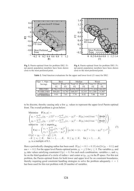
Fig. 3. Pareto-optimal front for problem DS2. Final
parent population members have been shown
close to the most preferred point.
F2
1.4
1.2
1
0.8
0.6
0.4
0.2
0
−0.2
Upper level
PO front
Most Preferred
Point
G=0
0 0.2 0.4 0.6 0.8 1 1.2 1.4
F1
Fig. 4. Pareto-optimal front for problem DS3. Final
parent population members have been shown
close to the most preferred point.
Table 2. Total function evaluations for the upper and lower level (21 runs) for DS2.
Algo. 1, Algo. 2, Best Median Worst
Savings Total LL Total UL Total LL Total UL Total LL Total UL
FE FE FE FE FE FE
HBLEMO 4,796,131 112,563 4,958,593 122,413 5,731,016 144,428
PI-HBLEMO 509,681 14,785 640,857 14,535 811,588 15,967
HBLEMO
P I−HBLEMO 9.41 7.61 7.74 8.42 7.06 9.05
to be discrete, thereby causing only a few y1 values to represent the upper level Pareto-optimal
front. The overall problem is given below:
⎛Minimize
F(x, y) =
⎝ y1 + K j=3 (yj − j/2) 2 + τ K i=3 (xi − yi) 2 − R(y1) cos(4 tan−1 y2−x2
y1−x1
y2 + K j=3 (yj − j/2) 2 + τ K i=3 (xi − yi) 2 − R(y1) sin(4 tan−1
y2−x2
y1−x1
⎞
⎠ ,
subject
to (x)
∈ argmin (x)
x1 +
f(x) =
K i=3 (xi − yi) 2
x2 + K i=3 (xi − yi) 2
g1(x) = (x1 − y1) 2 + (x2 − y2) 2 ≤ r2
,
G(y) = y2 − (1 − y2 1 ) ≥ 0,
−K ≤ xi ≤ K, for i = 1, . . . , K, 0 ≤ yj ≤ K, for j = 1, . . . , K,
y1 is a multiple of 0.1.
Here a periodically changing radius has been used: R(y1) = 0.1 + 0.15| sin(2π(y1 − 0.1)| and
use r = 0.2. For the upper level Pareto-optimal points, yi = j/2 for j ≤ 3. The variables y1 and
y2 take values satisfying constraint G(y) = 0. For each such combination, variables x1 and x2
lie on the third quadrant of a circle of radius r and center at (y1, y2) in the F-space. For this test
problem, the Pareto-optimal fronts for both lower and upper level lie on constraint boundaries,
thereby requiring good constraint handling strategies to solve the problem adequately. τ = 1
has been used for this test problem with 20 number of variables.
124
(7)