Progressively Interactive Evolutionary Multi-Objective Optimization ...

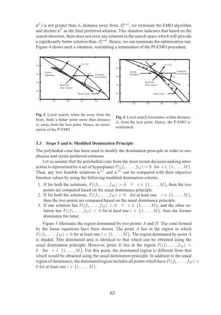
zT ) is not greater than ds distance away from Abest t , we terminate the EMO algorithm
and declare zT as the final preferred solution. This situation indicates that based on the
search direction, there does not exist any solution in the search space which will provide
a significantly better solution than Abest t . Hence, we can terminate the optimization run.
Figure 4 shows such a situation, warranting a termination of the PI-EMO procedure.
1
0.8
0.6
0.4
0.2
Current
Population
V1
Best Point
from Archive
V1+V2
Pareto Front
V2
Created by
Local Search
0
0 0.2 0.4 0.6 0.8 1
Fig. 3. Local search, when far away from the
front, finds a better point more than distance
ds away from the best point. Hence, no termination
of the P-EMO.
3.3 Steps 5 and 6: Modified Domination Principle
1
0.8
0.6
0.4
0.2
Current
Population
V1
Best Point
From Archive
Pareto Front
V1+V2
V2
Created by
Local Search
0
0 0.2 0.4 0.6 0.8 1
Fig. 4. Local search terminates within distance
ds from the best point. Hence, the P-EMO is
terminated.
The polyhedral cone has been used to modify the domination principle in order to emphasize
and create preferred solutions.
Let us assume that the polyhedral cone from the most recent decision-making interaction
is represented by a set of hyperplanes Pi(f1, . . . , fM ) = 0 for i ∈ {1, . . . , M}.
Then, any two feasible solutions x (1) and x (2) can be compared with their objective
function values by using the following modified domination criteria:
1. If for both the solutions, Pi(f1, . . . , fM ) > 0 ∀ i ∈ {1, . . . , M}, then the two
points are compared based on the usual dominance principle.
2. If for both the solutions, Pi(f1, . . . , fM) < 0 for at least one i ∈ {1, . . . , M},
then the two points are compared based on the usual dominance principle.
3. If one solution has Pi(f1, . . . , fM) > 0 ∀ i ∈ {1, . . . , M}, and the other solution
has Pi(f1, . . . , fM) < 0 for at least one i ∈ {1, . . . , M}, then the former
dominates the latter.
Figure 5 illustrates the region dominated by two points A and B. The cone formed
by the linear equations have been shown. The point A lies in the region in which
Pi(f1, . . . , fM) < 0 for at least one i ∈ {1, . . . , M}. The region dominated by point A
is shaded. This dominated area is identical to that which can be obtained using the
usual domination principle. However, point B lies in the region Pi(f1, . . . , fM) >
0 for i ∈ {1, . . . , M}. For this point, the dominated region is different from that
which would be obtained using the usual domination principle. In addition to the usual
region of dominance, the dominated region includes all points which have Pi(f1, . . . , fM) <
0 for at least one i ∈ {1, . . . , M}.
63