Progressively Interactive Evolutionary Multi-Objective Optimization ...

f 2
V(f)=V 2
A
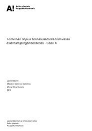
Fig. 6. Dominated regions of two points A and B using the modified
definition.
for the second-best member (P2 defined in the previous
subsection) from the set of η points given to the DM is
V2. Then, any two feasible solutions x (1) and x (2) can be
compared with their objective function values by using the
following modified domination criteria:
1. If both solutions have a value function value less than
V2, then the two points are compared based on the usual
dominance principle.
2. If both solutions have a value function value more than
V2, then the two points are compared based on the usual
dominance principle.
3. If one has value function value more than V2 and the
other has value function value less than V2, then the
former dominates the latter.
Figure 6 illustrates regions dominated by points A and B.
The value function contour having a value V2 is shown by
the curved line. Point A lies in the region in which the value
function is smaller than V2. The region dominated by point A
is shaded. This dominated area is identical to that which can be
obtained using the usual domination principle. However, point
B lies in the region in which the value function is larger than
V2. For this point, the dominated region is different from that
which would be obtained using the usual domination principle.
In addition to the usual region of dominance, the dominated
region includes all points which have a smaller value function
value than V2.
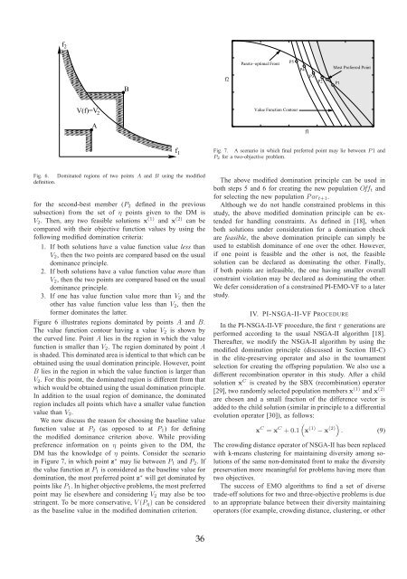
We now discuss the reason for choosing the baseline value
function value at P2 (as opposed to at P1) for defining
the modified dominance criterion above. While providing
preference information on η points given to the DM, the
DM has the knowledge of η points. Consider the scenario
in Figure 7, in which point z ∗ may lie between P1 and P2. If
the value function at P1 is considered as the baseline value for
domination, the most preferred point z ∗ will get dominated by
points like P1. In higher objective problems, the most preferred
point may lie elsewhere and considering V2 may also be too
stringent. To be more conservative, V (Pη) can be considered
as the baseline value in the modified domination criterion.
B
f 1
36
f2
Pareto−optimal Front
P5
Value Function Contour
P4
f1
P3
P2 P1
Most Preferred Point
Fig. 7. A scenario in which final preferred point may lie between P 1 and
P2 for a two-objective problem.
The above modified domination principle can be used in
both steps 5 and 6 for creating the new population Offt and
for selecting the new population P art+1.
Although we do not handle constrained problems in this
study, the above modified domination principle can be extended
for handling constraints. As defined in [18], when
both solutions under consideration for a domination check
are feasible, the above domination principle can simply be
used to establish dominance of one over the other. However,
if one point is feasible and the other is not, the feasible
solution can be declared as dominating the other. Finally,
if both points are infeasible, the one having smaller overall
constraint violation may be declared as dominating the other.
We defer consideration of a constrained PI-EMO-VF to a later
study.
IV. PI-NSGA-II-VF PROCEDURE
In the PI-NSGA-II-VF procedure, the first τ generations are
performed according to the usual NSGA-II algorithm [18].
Thereafter, we modify the NSGA-II algorithm by using the
modified domination principle (discussed in Section III-C)
in the elite-preserving operator and also in the tournament
selection for creating the offspring population. We also use a
different recombination operator in this study. After a child
solution x C is created by the SBX (recombination) operator
[29], two randomly selected population members x (1) and x (2)
are chosen and a small fraction of the difference vector is
added to the child solution (similar in principle to a differential
evolution operator [30]), as follows:
x C = x C + 0.1
x (1) − x (2)
. (9)
The crowding distance operator of NSGA-II has been replaced
with k-means clustering for maintaining diversity among solutions
of the same non-dominated front to make the diversity
preservation more meaningful for problems having more than
two objectives.
The success of EMO algorithms to find a set of diverse
trade-off solutions for two and three-objective problems is due
to an appropriate balance between their diversity maintaining
operators (for example, crowding distance, clustering, or other