Progressively Interactive Evolutionary Multi-Objective Optimization ...

maximum.
Maximize ǫ,
subject to Value Function Constraints
V (Pi) − V (Pj) ≥ ǫ, for all (i, j) pairs
satisfying Pi ≻ Pj,
|V (Pi) − V (Pj)| ≤ δV , for all (i, j) pairs
satisfying Pi ≡ Pj.
(4)
The first set of constraints ensure that the constraints specified
in the construction of the value function are met. It
includes variable bounds for the value function parameters
or any other equality or inequality constraints which need
to be satisfied to obtain feasible parameters for the value
function. The second and third set of constraints ensure
that the preference order specified by the decision maker
is maintained for each pair. The second set ensures the domination
of one point over the other such that the difference
in their values is at least ǫ. The third constraint set takes
into account all pairs of incomparable points. For such pairs
of points, we would like to restrict the absolute difference
between their value function values to be within a small
range (δV ). δV = 0.1ǫ has been used in the entire study
to avoid introducing another parameter in the optimization
problem. It is noteworthy that the value function optimization
task is considered to be successful, with all the preference
orders satisfied, only if a positive value of ǫ is obtained by
solving the above problem. A non-positive value of ǫ means
that the chosen value function is unable to fit the preference
information provided by the decision maker.
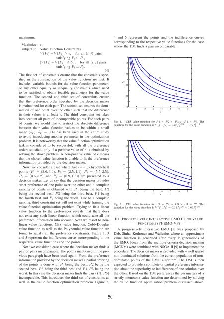
Now, we consider a case where five (η = 5) hypothetical
points (P1 = (3.6, 3.9), P2 = (2.5, 4.1), P3 = (5.5, 2.5),
P4 = (0.5, 5.2), and P5 = (6.9, 1.8)) are presented to a
decision maker. Let us say that the decision maker provides
strict preference of one point over the other and a complete
ranking of points is obtained with P1 being the best, P 2
being the second best, P 3 being the third best, P 4 being
the fourth best and P5 being the worst. Due to a complete
ranking, third constraint set will not exist while framing the
value function optimization problem. Trying to fit a linear
value function to the preferences reveals that there does
not exist any such linear function which could take all the
preference information into account. Next we resort to nonlinear
value functions. CES value function, Cobb-Douglas
value function as well as the Polynomial value function are
found to satisfy all the preference constraints. Figure 1, 3
and 5 represent the indifference curves corresponding to the
respective value functions and the points.
Next we consider a case where the decision maker finds a
pair or pairs incomparable. The points mentioned in the previous
paragraph have been used again. From the preference
information provided by the decision maker a partial ordering
of the points is done with P1 being the best, P 2 being the
second best, P 3 being the third best and P 4, P 5 being the
worst. In this case the decision maker finds the pair (P 4, P 5)
incomparable. This introduces the third set of constraints as
well in the value function optimization problem. Figure 2,
50
4 and 6 represent the points and the indifference curves
corresponding to the respective value functions for the case
where the DM finds a pair incomparable.
f 2
6
5.5
5
4.5
4
3.5
3
2.5
2
1.5
P4
P2
P1
1 2 3 4 5 6 7
f
1
Fig. 1. CES value function for P 1 ≻ P 2 ≻ P 3 ≻ P 4 ≻ P 5. The
equation for the value function is V (f1, f2) = 0.28f 0.13
1 + 0.72f 0.13
2
f 2
6
5.5
5
4.5
4
3.5
3
2.5
2
1.5
P4
P2
P1
1 2 3 4 5 6 7
f
1
Fig. 2. CES value function for P 1 ≻ P 2 ≻ P 3 ≻ P 4 ≡ P 5. The
equation for the value function is V (f1, f2) = 0.31f 0.26
1 + 0.69f 0.26
2
III. PROGRESSIVELY INTERACTIVE EMO USING VALUE
FUNCTIONS (PI-EMO-VF)
A progressively interactive EMO [1] was proposed by
Deb, Sinha, Korhonen and Wallenius where an approximate
value function is generated after every τ generations of
the EMO. Ideas from the multiple criteria decision making
(MCDM) were combined with NSGA-II [9] to implement the
procedure. The decision maker is provided with η well sparse
non-dominated solutions from the current population of nondominated
points of the EMO algorithm. The DM is then
expected to provide a complete or partial preference information
about the superiority or indifference of one solution over
the other. Based on the DM preferences the parameters of a
strictly monotone value function are determined by solving
the value function optimization problem discussed above.
P3
P3
P5
P5