Progressively Interactive Evolutionary Multi-Objective Optimization ...

eight differentproblems areshown. Acomparisonof theperformanceofthe proposed
algorithmwithour previously-proposedmethodology andwithanested optimization
strategy is made. The test problem construction procedure allowed us to create problemswhichexhibitconflictinggoalsbetweenlowerandupperleveloptimizationtasks.
The use of local searchand self-adaptivemethodologies enabledus to solve suchdifficult
problems using H-BLEMO, whereas these same problems arefound to be unsolvable
by our earlier methods. Further, a scalability study of the proposed algorithm is
made by considering different problem sizes ranging from 10 to 40 decision variables.
Finally, conclusions of the study arepresented.
2 Multi-Objective BilevelOptimization Problems
A multi-objective bilevel optimization problem has two levels of multi-objective optimization
problems such that a feasible solution of the upper level problem must be a
member of the Pareto-optimal set of the lower level optimization problem. A general
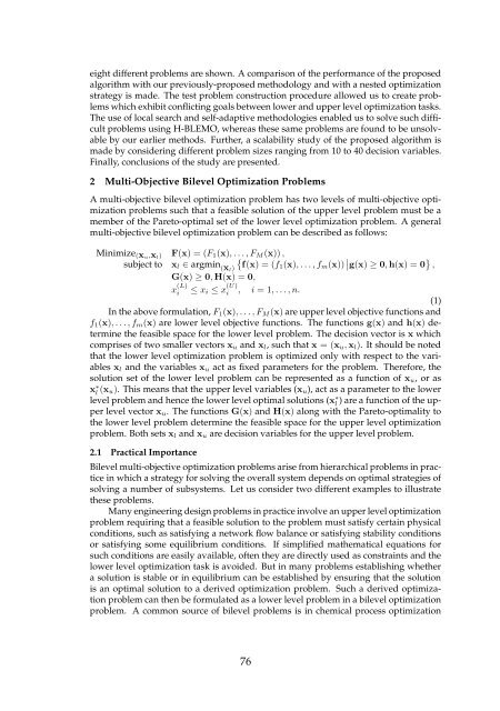
multi-objective bilevel optimizationproblemcanbe describedas follows:
Minimize (xu,xl) F(x) = (F1(x), . . . , FM
(x)) ,
subject to xl ∈ argmin (xl) f(x) = (f1(x), . . . , fm(x))
g(x) ≥ 0, h(x) = 0 ,
G(x) ≥ 0, H(x) = 0,
≤ xi ≤ x (U)
i , i = 1, . . . , n.
x (L)
i
(1)
Intheaboveformulation, F1(x), . . . , FM (x)areupperlevelobjectivefunctionsand
f1(x), . . . , fm(x) are lower level objective functions. The functions g(x) and h(x) determine
the feasible space for the lower level problem. The decision vector is x which
comprises of two smaller vectors xu and xl, such that x = (xu, xl). It should be noted
that the lower level optimization problem is optimized only with respect to the variables
xl and the variables xu act as fixed parameters for the problem. Therefore, the
solution set of the lower level problem can be represented as a function of xu, or as
x ∗ l (xu). This means that the upper level variables (xu), act as a parameter to the lower
levelproblemandhencethelowerleveloptimalsolutions (x ∗ l )areafunctionoftheupper
level vector xu. The functions G(x) and H(x) along with the Pareto-optimality to
the lower level problem determine the feasible space for the upper level optimization
problem. Bothsets xl and xu aredecisionvariablesfor the upperlevelproblem.
2.1 PracticalImportance
Bilevelmulti-objectiveoptimizationproblemsarisefromhierarchicalproblemsinpracticeinwhichastrategyforsolving
theoverallsystemdependsonoptimalstrategiesof
solving a number of subsystems. Let us consider two different examples to illustrate
these problems.
Manyengineeringdesignproblemsinpracticeinvolveanupperleveloptimization
problem requiring that a feasible solution to the problem must satisfy certain physical
conditions, such as satisfying a network flow balance or satisfying stability conditions
or satisfying some equilibrium conditions. If simplified mathematical equations for
such conditions are easily available,often they aredirectly used as constraints and the
lower level optimization task is avoided. But in many problems establishing whether
a solution is stable or in equilibrium can be established by ensuring that the solution
is an optimal solution to a derived optimization problem. Such a derived optimizationproblemcanthenbeformulatedasalowerlevelprobleminabileveloptimization
problem. A common source of bilevel problems is in chemical process optimization
76