Progressively Interactive Evolutionary Multi-Objective Optimization ...

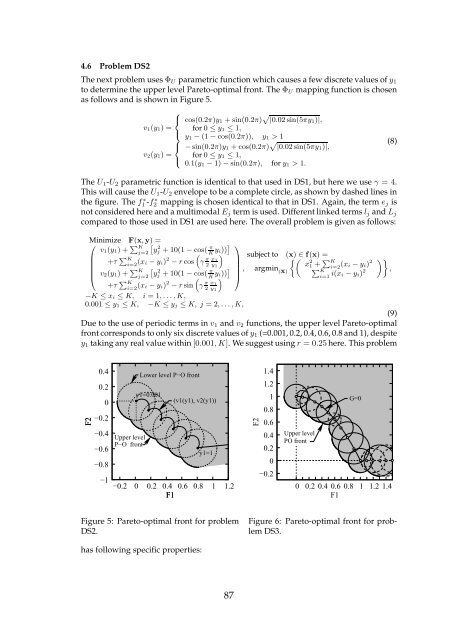
4.6 ProblemDS2
Thenextproblemuses ΦU parametricfunctionwhichcausesafewdiscretevaluesof y1
todeterminethe upperlevelPareto-optimalfront. The ΦU mappingfunctionis chosen
asfollows and is shown inFigure5.
⎧
⎨
v1(y1) =
⎩
⎧
⎨
v2(y1) =
⎩
cos(0.2π)y1 + sin(0.2π) |0.02 sin(5πy1)|,
for 0 ≤ y1 ≤ 1,
y1 − (1 − cos(0.2π)), y1 > 1
− sin(0.2π)y1 + cos(0.2π) |0.02 sin(5πy1)|,
for 0 ≤ y1 ≤ 1,
0.1(y1 − 1) − sin(0.2π), for y1 > 1.
The U1-U2 parametric function is identical to that used in DS1, but here we use γ = 4.
This will causethe U1-U2 envelopetobeacompletecircle,asshown bydashedlines in
the figure. The f ∗ 1-f ∗ 2 mapping is chosen identical to that in DS1. Again, the term ej is
notconsideredhereandamultimodal Ej termisused. Differentlinkedterms lj and Lj
comparedto those used inDS1areused here. The overallproblemis givenas follows:
Minimize F(x, y) =
⎛
⎜
⎝
v1(y1) + K 2
j=2 yj + 10(1 − cos( π
+τ K i=2 (xi − yi)2
− r cos γ π x1
2 y1
v2(y1) + K 2
j=2 yj + 10(1 − cos( π
+τ K
i=2 (xi − yi)2 − r sin
γ π
2
K yi))
K yi))
⎞
⎟
⎠ ,
subject to (x)
∈ f(x) =
2
x1 +
argmin (x)
K i=2 (xi − yi)2
K i=1 i(xi − yi)2
x1
y1
−K ≤ xi ≤ K, i = 1, . . . , K,
0.001 ≤ y1 ≤ K, −K ≤ yj ≤ K, j = 2, . . . , K,
(8)
,
(9)
Due tothe use of periodic terms in v1 and v2 functions, the upper level Pareto-optimal
frontcorrespondstoonlysixdiscretevaluesof y1(=0.001,0.2,0.4,0.6,0.8and1),despite
y1takinganyrealvaluewithin [0.001, K]. Wesuggestusing r = 0.25here. Thisproblem
F2
0.4
0.2
0
−0.2
−0.4
−0.6
−0.8
−1
Upper level
P−O front
−0.2
Lower level P−O front
y1=0.001
0
(v1(y1), v2(y1))
0.2 0.4 0.6 0.8
F1
y1=1
1
1.2
Figure 5: Pareto-optimal front for problem
DS2.
has following specific properties:
87
F2
1.4
1.2
1
0.8
0.6
0.4
0.2
0
−0.2
Upper level
PO front
G=0
0 0.2 0.4 0.6 0.8 1 1.2 1.4
F1
Figure 6: Pareto-optimal front for problemDS3.