An Analysis on Danish Micro Data - School of Economics and ...
An Analysis on Danish Micro Data - School of Economics and ...
An Analysis on Danish Micro Data - School of Economics and ...
You also want an ePaper? Increase the reach of your titles
YUMPU automatically turns print PDFs into web optimized ePapers that Google loves.
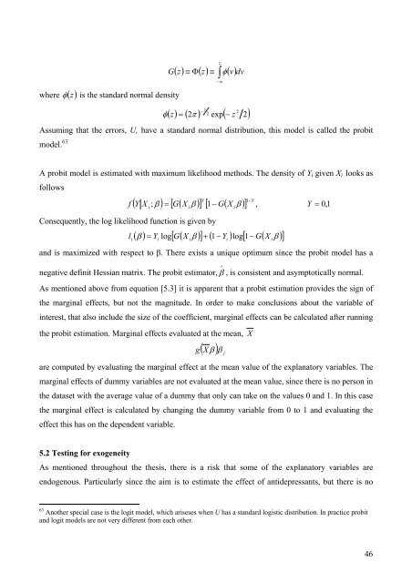
where φ ( z)<br />
is the st<strong>and</strong>ard normal density<br />
φ<br />
( z)<br />
≡ Φ(<br />
z)<br />
≡ ( v)<br />
z<br />
∫ ∞<br />
−<br />
G φ<br />
dv<br />
− 1<br />
2<br />
( z) = ( 2π<br />
) 2 exp(<br />
− z 2)<br />
Assuming that the errors, U, have a st<strong>and</strong>ard normal distributi<strong>on</strong>, this model is called the probit<br />
model. 63<br />
A probit model is estimated with maximum likelihood methods. The density <strong>of</strong> Yi given Xi looks as<br />
follows<br />
f<br />
( Y X ; ) G(<br />
X β )<br />
i<br />
Y<br />
1−Y [ ] [ 1−<br />
G(<br />
X ) ] ,<br />
C<strong>on</strong>sequently, the log likelihood functi<strong>on</strong> is given by<br />
β = β<br />
Y = 0,<br />
1<br />
i<br />
( ) = Y log [ G(<br />
X β ) ] + ( 1−<br />
Y ) log[<br />
1 G(<br />
X β ) ]<br />
l −<br />
i β i<br />
i<br />
i<br />
i<br />
<strong>and</strong> is maximized with respect to β. There exists a unique optimum since the probit model has a<br />
negative definit Hessian matrix. The probit estimator, ∧<br />
β , is c<strong>on</strong>sistent <strong>and</strong> asymptotically normal.<br />
As menti<strong>on</strong>ed above from equati<strong>on</strong> [5.3] it is apparent that a probit estimati<strong>on</strong> provides the sign <strong>of</strong><br />
the marginal effects, but not the magnitude. In order to make c<strong>on</strong>clusi<strong>on</strong>s about the variable <strong>of</strong><br />
interest, that also include the size <strong>of</strong> the coefficient, marginal effects can be calculated after running<br />
the probit estimati<strong>on</strong>. Marginal effects evaluated at the mean, X<br />
( Xβ<br />
) j<br />
g β<br />
are computed by evaluating the marginal effect at the mean value <strong>of</strong> the explanatory variables. The<br />
marginal effects <strong>of</strong> dummy variables are not evaluated at the mean value, since there is no pers<strong>on</strong> in<br />
the dataset with the average value <strong>of</strong> a dummy that <strong>on</strong>ly can take <strong>on</strong> the values 0 <strong>and</strong> 1. In this case<br />
the marginal effect is calculated by changing the dummy variable from 0 to 1 <strong>and</strong> evaluating the<br />
effect this has <strong>on</strong> the dependent variable.<br />
5.2 Testing for exogeneity<br />
As menti<strong>on</strong>ed throughout the thesis, there is a risk that some <strong>of</strong> the explanatory variables are<br />
endogenous. Particularly since the aim is to estimate the effect <strong>of</strong> antidepressants, but there is no<br />
63 <str<strong>on</strong>g>An</str<strong>on</strong>g>other special case is the logit model, which ariseses when U has a st<strong>and</strong>ard logistic distributi<strong>on</strong>. In practice probit<br />
<strong>and</strong> logit models are not very different from each other.<br />
i<br />
46


