Projects - Cengage Learning

C-106 Appendix C
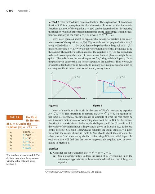
Method 2 This method uses function iteration. The explanation of iteration in
Section 3.5* is a prerequisite for this discussion. It turns out that for certain
functions f, a root of the equation x f(x) can be determined just by iterating
the function f with an appropriate initial input. (Note that our tree-cutting equation
was initially in the form x f(x); it was x 1 3 12 x. )
We’ll use Figures A and B to explain why iterating a function f can determine
a root of the equation x f(x). Figure A shows the graph of a function f,
along with the line y x. Let (r, r) denote the point where the graph of y f(x)
intersects the line y x. (Why do the two coordinates of that point have to be
the same?) The number r is then a root of the equation x f(x). We would like
to be able to compute the value of r to as many decimal places as might be required.
Figure B shows the iteration process for f using an initial input x 0 . From
the pattern you can see that the iterates approach the number r. Thus we can, in
principle at least, determine the root r to as many decimal places as we want by
carrying out the iteration process sufficiently many times.
y
y=x
y
y=x
y=ƒ
y=ƒ
r
x
r
x¸
x
TABLE 1 The First
Six Iterates
of x 0 5 Under the
3
Function f(x) 112 x
x 1 1.91293 . . .
x 2 2.16066 . . .
x 3 2.14283 . . .
x 4 2.14412 . . .
x 5 2.14403 ...
x 6 2.14404 ...
The numbers are not rounded. The
digits in cyan show the agreement
with the value obtained using
Method 1.
Figure A
Figure B
Now let’s see how this works in the case of Fior’s tree-cutting equation
x 1 3 12 x. The function to be iterated is f(x) 1 3 12 x. We need an initial
input x 0 . In general, one first makes an estimate of what the root might be
and then uses that estimate or something close to it for x 0 . But for the present
function f, a remarkable fact is that any initial input x 0 will do. (A case in which
the choice of the initial input is important is given in Exercise 1(c) at the end
of this project.) Selecting (somewhat at random) the initial input x 0 5 now,
we obtain the results shown in Table 1. You should check the entries in this
table yourself and then set up similar tables using different initial inputs. In
each case you will find that the iterates approach the required root, as determined
in Method 1.
Exercises
1. Consider the cubic equation g(x) x 3 6x 2 0.
(a) Use a graphing utility to draw the graph of g. By zooming in on the
x-intercept, approximate to the nearest hundredth the root of the given
equation.
*Precalculus: A Problems-Oriented Approach, 7th edition