Option-Implied Currency Risk Premia - Princeton University

A
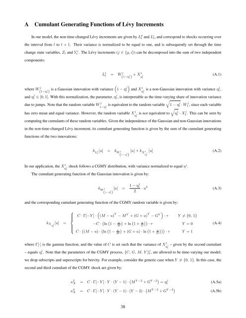
Cumulant Generating Functions of Lévy Increments
In our model, the non-time-changed Lévy increments are given by L g t and L i t, and correspond to shocks occurring over
the interval from t to t + 1. Their variance is normalized to be equal to one, and is subsequently set through the time
change state variables, Z t and Y i
t . The Lévy increments (j ∈ {g, i}) can be decomposed into the sum of two independent
components:
L j t = W j (1−ηt) + j Xj η j t
)
where W
(1 j
(1−ηt) is a Gaussian innovation with variance − η j j t and X j η j t
(A.1)
is a non-Gaussian innovation with variance η j t ,
and η j t ∈ [0, 1]. With this normalization, the parameter, η j t , is interpretable as the time-varying share of innovation variance
√
due to jumps. Note that the random variable W j is equivalent to the random variable 1 − η j 1−η j t · W j 1 , since each variable
t
√
has zero mean and equal variance. However, the random variable X j is not equivalent to η j η j t · X j 1 . This can be seen by
t
computing the cumulants of these random variables. Given the independence of the Gaussian and non-Gaussian innovations
in the non-time-changed Lévy increment, its cumulant generating function is given by the sum of the cumulant generating
functions of the two innovations:
k L
j [u] = k
t
W
j
( 1−η
t) [u] + k j X j [u]
η j t
(A.2)
In our application, the X j η j t
shock follows a CGMY distribution, with variance normalized to equal η j .
The cumulant generating function of the Gaussian innovation is given by:
k W
j
( 1−η j t) [u] = 1 − ηj t
2
· u 2 (A.3)
and the corresponding cumulant generating function of the CGMY random variable is given by:
k Xη j
[u] =
t
⎧
⎪⎨
⎪⎩
)
C · Γ[−Y ] ·
((M − u) Y − M Y + (G + u) Y − G Y · τ Y ≠ {0, 1}
−C · (ln ( ) (
1 − u M + ln 1 +
u
G))
· τ Y = 0
(A.4)
C · ((M
− u) · (ln ( ) ( )))
1 − u M + (G + u) · ln 1 +
u
G · τ Y = 1
where Γ[·] is the gamma function, and the value of C is set such that the variance of X j η j t
– given by the second cumulant
– equals η j t . Note that the parameters of the CGMY process, {C, G, M, Y } j t, are allowed to be time-varying our model;
we drop subscripts and superscripts for brevity. For example, consider the generic case when Y ≠ {0, 1}. In this case, the
second and third cumulant of the CGMY shock are given by:
κ 2 X = C · Γ[−Y ] · Y · (Y − 1) · (M Y −2 + G Y −2) = η j t (A.5a)
κ 3 X = C · Γ[−Y ] · Y · (Y − 1) · (Y − 2) · (M Y −3 + G Y −3) (A.5b)
38