Option-Implied Currency Risk Premia - Princeton University
Option-Implied Currency Risk Premia - Princeton University
Option-Implied Currency Risk Premia - Princeton University
You also want an ePaper? Increase the reach of your titles
YUMPU automatically turns print PDFs into web optimized ePapers that Google loves.
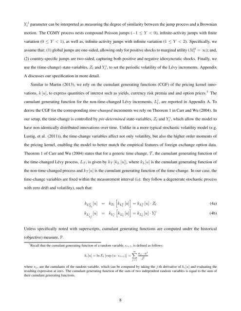
Y j<br />
t parameter can be interpreted as measuring the degree of similarity between the jump process and a Brownian<br />
motion. The CGMY process nests compound Poisson jumps (−1 ≤ Y < 0), infinite-activity jumps with finite<br />
variation (0 ≤ Y < 1), as well as, infinite-activity jumps with infinite variation (1 ≤ Y < 2). Specifically, we<br />
assume that: (1) global jumps are one-sided, allowing only for positive shocks to marginal utility (M g t<br />
= ∞); and,<br />
(2) country-specific jumps are two-sided, capturing both positive and negative idiosyncratic shocks. Finally, we<br />
use the (time-change) state-variables, Z t and Y i<br />
t , to set the periodic volatility of the Lévy increments. Appendix<br />
A discusses our specification in more detail.<br />
Similar to Martin (2013), we rely on the cumulant generating functions (CGF) of the pricing kernel innovations,<br />
k [u], to express quantities of interest such as yields, currency risk premia and and option prices. 7 The<br />
cumulant generating function for the non-time-changed Lévy increments, L j t , are reported in Appendix A. To<br />
derive the CGF for the corresponding time-changed increments we rely on Theorem 1 in Carr and Wu (2004). In<br />
our setup, the time-change is controlled by pre-determined state-variables, Z t and Y i<br />
t , which allow the model to<br />
have non-identically distributed innovations over time. Unlike in a more typical stochastic volatility model (e.g.<br />
Lustig, et al. (2011)), the time-change variables affect not only volatility, but also the higher order moments of<br />
the pricing kernel, enabling the model to better match the empirical features of foreign exchange option data.<br />
Theorem 1 of Carr and Wu (2004) states that for a generic time change, T , the cumulant generating function of<br />
the time-changed Lévy process, L T , is given by k T [k L [u]], where k L [u] is the cumulant generating function of<br />
the non-time-changed process and k T [u] is the cumulant generating function of the time-change. In our case, the<br />
time-change variables are fixed within the measurement interval (i.e. they follow a degenerate stochastic process<br />
with zero drift and volatility), such that:<br />
[ ]<br />
k L<br />
g [u] = k Zt k<br />
Z L<br />
g [u]<br />
t t<br />
k L i<br />
Y i<br />
t<br />
[u] = k Y i<br />
t<br />
k L i<br />
t<br />
[u]<br />
[<br />
]<br />
= k L<br />
g<br />
t [u] · Z t<br />
= k L i<br />
t<br />
[u] · Y i<br />
t<br />
(4a)<br />
(4b)<br />
Unless specifically noted with superscripts, cumulant generating functions are computed under the historical<br />
(objective) measure, P.<br />
7 Recall that the cumulant generating function of a random variable, ɛ t+1, is defined as follows:<br />
k ɛ[u] = ln E t [exp (u · ɛ t+1)] =<br />
∞∑ κ j · u j<br />
where κ j, are the cumulants of the random variable, which can be computed by taking the j-th derivative of k ɛ[u] and evaluating the<br />
resulting expression at zero. The cumulant generating function of the sum of two independent random variables is equal to the sum of<br />
their cumulant generating functions.<br />
j=1<br />
j!<br />
8


