Option-Implied Currency Risk Premia - Princeton University

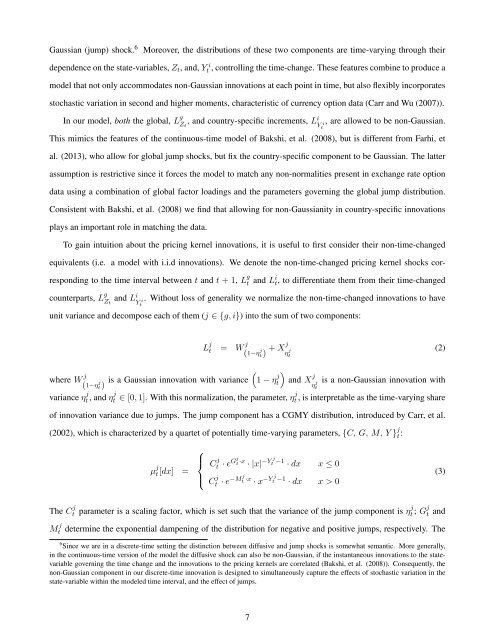
Gaussian (jump) shock. 6
Moreover, the distributions of these two components are time-varying through their
dependence on the state-variables, Z t , and, Y i
t , controlling the time-change. These features combine to produce a
model that not only accommodates non-Gaussian innovations at each point in time, but also flexibly incorporates
stochastic variation in second and higher moments, characteristic of currency option data (Carr and Wu (2007)).
In our model, both the global, L g Z t
, and country-specific increments, L i , are allowed to be non-Gaussian.
Yt
i
This mimics the features of the continuous-time model of Bakshi, et al. (2008), but is different from Farhi, et
al. (2013), who allow for global jump shocks, but fix the country-specific component to be Gaussian. The latter
assumption is restrictive since it forces the model to match any non-normalities present in exchange rate option
data using a combination of global factor loadings and the parameters governing the global jump distribution.
Consistent with Bakshi, et al. (2008) we find that allowing for non-Gaussianity in country-specific innovations
plays an important role in matching the data.
To gain intuition about the pricing kernel innovations, it is useful to first consider their non-time-changed
equivalents (i.e. a model with i.i.d innovations). We denote the non-time-changed pricing kernel shocks corresponding
to the time interval between t and t + 1, L g t and Li t, to differentiate them from their time-changed
counterparts, L g Z t
and L i . Without loss of generality we normalize the non-time-changed innovations to have
Yt
i
unit variance and decompose each of them (j ∈ {g, i}) into the sum of two components:
L j t = W j (1−ηt) + j Xj η j t
)
where W
(1 j
(1−ηt) is a Gaussian innovation with variance − η j j t and X j η j t
(2)
is a non-Gaussian innovation with
variance η j t , and ηj t ∈ [0, 1]. With this normalization, the parameter, ηj t , is interpretable as the time-varying share
of innovation variance due to jumps. The jump component has a CGMY distribution, introduced by Carr, et al.
(2002), which is characterized by a quartet of potentially time-varying parameters, {C, G, M, Y } j t :
µ j t [dx] = ⎧
⎪⎨
⎪ ⎩
C j t · eGj t ·x · |x| −Y j
t −1 · dx x ≤ 0
C j t · e−M j t ·x · x −Y j
t −1 · dx x > 0
(3)
The C j t parameter is a scaling factor, which is set such that the variance of the jump component is ηj t ; Gj t and
M j t
determine the exponential dampening of the distribution for negative and positive jumps, respectively. The
6 Since we are in a discrete-time setting the distinction between diffusive and jump shocks is somewhat semantic. More generally,
in the continuous-time version of the model the diffusive shock can also be non-Gaussian, if the instantaneous innovations to the statevariable
governing the time change and the innovations to the pricing kernels are correlated (Bakshi, et al. (2008)). Consequently, the
non-Gaussian component in our discrete-time innovation is designed to simultaneously capture the effects of stochastic variation in the
state-variable within the modeled time interval, and the effect of jumps.
7