arbres aléatoires, conditionnement et cartes planaires - DMA - Ens

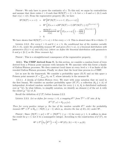
Proof : We only have to prove the continuity of v. To this end, we argue by contradiction
and assume that there exists t > 0 such that Θ(H(T ) = t) > 0. Let s > 0 and u ∈ (0,t) such
that v(u) > v(t). From the regenerative property (R), we have
Θ s (H(T ) = s + t) = Θ s( )
Θ s (H(T ) = s + t | Z(s,s + u))
= Θ s ( Z(s,s + u)Θ u (H(T ) = t)(Θ u (H(T ) ≤ t)) Z(s,s+u)−1)
=
> 0.
Θ(H(T ) = t)
v(u)
(
Θ
(Z(s,s s + u) 1 − v(t) ) )
Z(s,s+u)−1
v(u)
We have shown that Θ(H(T ) = t + s) > 0 for every s > 0. This is absurd since Θ is σ-finite. □
Lemma 2.3.2. For every t > 0 and 0 < a < b, the conditional law of the random variable
Z(t,t+b), under the probability measure Θ t and given Z(t,t+a), is a binomial distribution with
parameters Z(t,t+a) and v(b)/v(a) (where we define the binomial distribution with parameters
0 and p ∈ [0,1] as the Dirac measure δ 0 ).
Proof : This is a straightforward consequence of the regenerative property.
□
2.3.1. The CSBP derived from Θ. In this section, we consider a random forest of trees
derived from a Poisson point measure with intensity Θ. We associate with this forest a family
of Galton-Watson processes. We then construct local times at every level a > 0 as limits of the
rescaled Galton-Watson processes. Finally we show that the local time process is a CSBP.
Let us now fix the framework. We consider a probability space (Ω, P) and on this space a
Poisson point measure N = ∑ i∈I δ T i
on T, whose intensity is the measure Θ.
2.3.1.1. A family of Galton-Watson trees. We start with some notation that we need in
the first lemma. We consider on another probability space (Ω ′ , P ′ ), a collection (θ ξ ,ξ ∈ A) of
independent A-valued random variables such that for every ξ ∈ A, θ ξ is distributed uniformly
overÔ−1 (ξ). In what follows, to simplify notation, we identify an element ξ of the set A with
the subsetÔ−1 (ξ) of A.
Recall the definition of ξ ε (T ) before Lemma 2.2.2.
Lemma 2.3.3. Let us define for every ε > 0, a mapping θ (ε) from T (ε) × Ω ′ into A by
θ (ε) (T ,ω) = θ ξ ε (T )(ω).
Then for every positive integer p, the law of the random variable θ (ε) under the probability
measure Θ pε ⊗ P ′ is Π µε (· | H(θ) ≥ p − 1) where µ ε denotes the law of Z(ε,2ε) under Θ ε .
Proof : Since {H(T ) > pε} × Ω ′ = {H(θ (ε) ) ≥ p − 1} for every p ≥ 1, it suffices to show
the result for p = 1. Let k be a nonnegative integer. According to the construction of ξ ε (T ), we
have
( Θ ε ⊗ P ′ k ∅
(θ (ε)) )
= k = Θ ε (Z(ε,2ε) = k) = µ ε (k).
36