arbres alÃ©atoires, conditionnement et cartes planaires - DMA - Ens

More documents

Recommendations

Info

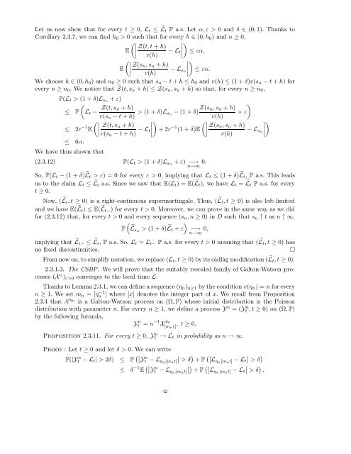
Let us now show that for every t ≥ 0, L t ≤ ˜L t P a.s. Let α,ε > 0 and δ ∈ (0,1). Thanks to Corollary 2.3.7, we can find h 0 > 0 such that for every h ∈ (0,h 0 ) and n ≥ 0, (∣ ∣) ∣∣∣ Z(t,t + h) ∣∣∣ E − L t ≤ εα, v(h) (∣ ∣) ∣∣∣ Z(s n ,s n + h) ∣∣∣ E − L sn ≤ εα. v(h) We choose h ∈ (0,h 0 ) and n 0 ≥ 0 such that s n − t + h ≤ h 0 and v(h) ≤ (1 + δ)v(s n − t + h) for every n ≥ n 0 . We notice that Z(t,s n + h) ≤ Z(s n ,s n + h) so that, for every n ≥ n 0 , P(L t > (1 + δ)L sn + ε) ( ≤ P L t − Z(t,s n + h) v(s n − t + h) > (1 + δ)L s n − (1 + δ) Z(s ) n,s n + h) + ε v(h) (∣ ) (∣ ∣) ∣∣∣ ≤ 2ε −1 Z(t,s n + h) E v(s n − t + h) − L ∣∣∣ t∣ + 2ε −1 Z(s n ,s n + h) ∣∣∣ (1 + δ)E − L sn v(h) ≤ 6α. We have thus shown that (2.3.12) P(L t > (1 + δ)L sn + ε) −→ n→∞ 0. So, P(L t − (1 + δ) ˜L t > ε) = 0 for every ε > 0, implying that L t ≤ (1 + δ) ˜L t , P a.s. This leads us to the claim L t ≤ ˜L t a.s. Since we saw that E(L t ) = E( ˜L t ), we have L t = ˜L t P a.s. for every t ≥ 0. Now, ( ˜L t ,t ≥ 0) is a right-continuous supermartingale. Thus, ( ˜L t ,t ≥ 0) is also left-limited and we have E( ˜L t ) ≤ E( ˜L t− ) for every t > 0. Moreover, we can prove in the same way as we did for (2.3.12) that, for every t > 0 and every sequence (s n ,n ≥ 0) in D such that s n ↑ t as n ↑ ∞, ( P ˜Lsn > (1 + δ) ˜L ) t + ε −→ 0, n→∞ implying that ˜L t− ≤ ˜L t , P a.s. So, L t = L t− P a.s. for every t > 0 meaning that ( ˜L t ,t ≥ 0) has no fixed discontinuities. □ From now on, to simplify notation, we replace (L t ,t ≥ 0) by its càdlàg modification ( ˜L t ,t ≥ 0). 2.3.1.3. The CSBP. We will prove that the suitably rescaled family of Galton-Watson processes (X ε ) ε>0 converges to the local time L. Thanks to Lemma 2.3.1, we can define a sequence (η n ) n≥1 by the condition v(η n ) = n for every n ≥ 1. We set m n = [ηn −1 ] where [x] denotes the integer part of x. We recall from Proposition 2.3.4 that X ηn is a Galton-Watson process on (Ω, P) whose initial distribution is the Poisson distribution with parameter n. For every n ≥ 1, we define a process Y n = (Yt n ,t ≥ 0) on (Ω, P) by the following formula, Yt n = n −1 X ηn [m , t ≥ 0. nt] Proposition 2.3.11. For every t ≥ 0, Y n t → L t in probability as n → ∞. Proof : Let t ≥ 0 and let δ > 0. We can write P(|Yt n − L t| > 2δ) ≤ P (∣ ) (∣ ∣ ) ∣ Y n t − L ηn[m ∣ nt] > δ + P ∣Lηn[m nt] − L t > δ ≤ δ −1 E (∣ ∣ Y n t − L ηn[m ∣ ) nt] + P (∣ ∣ ) ∣ Lηn[mnt] − L t > δ . 42
Now, Corollary 2.3.7 and Proposition 2.3.8 imply respectively that E (∣ ∣Yt n − L ∣ ) η n[m nt] −→ which completes the proof. n→∞ 0, P (∣ ∣L ηn[m nt] − L t ∣ ∣ > δ ) −→ n→∞ 0, Corollary 2.3.12. For every t ≥ 0, the law of Y n t under P(· | X ηn 0 = n) converges weakly to the law of L t under P as n → ∞. Proof : For positive integers n and k, we denote by µ n the offspring distribution of the Galton-Watson process X ηn , by f n the generating function of µ n and by fk n the k-th iterate fk n = fn ◦ ... ◦ f n of f n . Let λ > 0 and t ≥ 0. We have, ∞ E(exp(−λYt n )) = ∑ ( e −nnp f[m n p! nt] (e −λ/n)) p ( ( ( = exp −n 1 − f[m n nt] e −λ/n))) . p=0 From Proposition 2.3.11, it holds that ( ( ( exp −n 1 − f[m n nt] e −λ/n))) −→ E(exp(−λL t )). n→∞ Let us set u(t,λ) = − log(E[exp(−λL t )]). It follows that, ( ( n 1 − f[m n nt] e −λ/n)) −→ u(t,λ). n→∞ Thus, we obtain, ( ) E exp(−λYt n ) ∣ X ηn 0 = n = ( ( f[m n nt] e −λ/n)) n −→ exp(−u(t,λ)) = E[exp(−λL t )]. n→∞ At this point, we can use Theorem 2.2.1 to assert that (L t ,t ≥ 0) is a CSBP and that the law of (Yt n ,t ≥ 0) under the probability measure P(· | X ηn 0 = n) converges to the law of (L t ,t ≥ 0) as n → ∞ in the space of probability measures on the Skorokhod space D(R + ). To verify the assumptions of Theorem 2.2.1, we need to check that there exists δ > 0 such that P(L δ > 0) > 0. This is obvious from Lemma 2.3.9. 2.3.2. Identification of the measure Θ. In the previous section, we have constructed from Θ a CSBP L, which becomes extinct almost surely. We denote by ψ the associated branching mechanism. We can consider the σ-finite measure Θ ψ , which is the law of the Lévy tree associated with L. Our goal is to show that the measures Θ and Θ ψ coincide. Recall that µ n denotes the offspring distribution of the Galton-Watson process X ηn . Lemma 2.3.13. For every a > 0, the law of the R-tree η n T θ under Π µ n(· | H(θ) ≥ [am n ]) converges as n → ∞ to the probability measure Θ ψ (· | H(T ) > a) in the sense of weak convergence of measures in the space T. Proof : We first check that, for every δ > 0, (2.3.13) lim inf n→∞ P(Yn δ = 0) > 0. Indeed, we have ) ( ) P(Yδ (N(H(T n = 0) = P ) > ([m n δ] + 1)η n ) = 0 = exp − v(([m n δ] + 1)η n ) . □ □ 43
Page 1: THÈSE DE DOCTORAT DE L’UNIVERSIT
Page 5: Table des matières Chapitre 1. Int
Page 8 and 9: t ∈ [0,2(#A − 1)] entier, on d
Page 10 and 11: Remarquons qu’un arbre planaire p
Page 12 and 13: Théorème 1.2.2. Soit Θ une mesur
Page 14 and 15: Rappelons que si s ∈ [0,1], alors
Page 16 and 17: On définit ensuite W [s] à partir
Page 18 and 19: 1.5. Arbres spatiaux et cartes plan
Page 20 and 21: Si de plus U v ≥ 1 pour tout v
Page 22 and 23: Fig. 2. Construction d’une carte
Page 24 and 25: Théorème 1.6.2. Soit q une suite
Page 27 and 28: CHAPITRE 2 Regenerative real trees
Page 29 and 30: andom ordering to the discrete tree
Page 31 and 32: 2.2.2.1. The space (T,GH) of rooted
Page 33 and 34: first generation. Then, if F : A k
Page 35 and 36: Let us now set I t = inf {X s : 0
Page 37 and 38: Let us fix k ≥ 1 with µ ε (k) >
Page 39 and 40: The bound (2.3.6) implies ( ∑ ∞
Page 41: Now, thanks to Proposition 2.3.6,
Page 45 and 46: Proposition 2.4.4. For every ε > 0
Page 47 and 48: Since f is bounded and Xu 1/n ≤ L
Page 49: where θ 1 ,... ,θ p denote the co
Page 52 and 53: This definition should become clear
Page 54 and 55: the geometric distribution, this gi
Page 56 and 57: Brownian motion in [0, ∞[ started
Page 58 and 59: for every u ∈ T and l ∈ [0,h u
Page 60 and 61: if r ∈ [0,σ], and Ŵ r [s] = 0 i
Page 62 and 63: where the last equality follows fro
Page 64 and 65: where c(ε,δ) = N q (B ε,δ ) doe
Page 66 and 67: Similarly, N 0 (½{W>−ε}e −σ
Page 68 and 69: To simplify notation, we have writt
Page 70 and 71: N = ∑ i∈I δ ω i with intensit
Page 72 and 73: It remains to study ε −4 N 0 (½
Page 74 and 75: Proof of Theorems 3.1.1 and 3.1.2 :
Page 76 and 77: For every h > 0, we set N h 0 = N 0
Page 78 and 79: Now note that the range of the Brow
Page 80 and 81: and conditionally given W α , the
Page 82 and 83: for every i ∈ I and s ≥ 0. For
Page 84 and 85: and then, for every u ∈ T \{∅},
Page 86 and 87: Q θ ε As a consequence of Lemma 3
Page 88 and 89: From (3.5.3) and Lemma 3.5.3, it th
Page 90 and 91: ipartite planar maps are in one-to-
Page 92 and 93:
Let us turn to the special case of
Page 94 and 95:
Write P for the probability measure
Page 96 and 97:
From [43], we know that µ 1 has sm
Page 98 and 99:
(ii) The law of the random measure
Page 100 and 101:
which means that k is the time of t
Page 102 and 103:
4.3.2. Estimates for the probabilit
Page 104 and 105:
Proof : The proof of this lemma is
Page 106 and 107:
Recall that p ≥ 1 is such that µ
Page 108 and 109:
such that each pair (T n ,U n ) is
Page 110 and 111:
Then, under the probability measure
Page 112 and 113:
Let us now define on the event E n
Page 114 and 115:
which implies together with (4.3.29
Page 116 and 117:
measure I n defined by 〈I n ,g〉
Page 118 and 119:
Lemma 4.4.3. Let (T ,U) ∈ T mob 1
Page 120 and 121:
where the last bound follows from a
Page 122 and 123:
However we can find β > 0, γ > 0
Page 124:
[25] Evans, S.N., Winter, A. Subtre
show all

arbres alÃ©atoires, conditionnement et cartes planaires - DMA - Ens

Create successful ePaper yourself

Delete template?

Save as template?