arbres aléatoires, conditionnement et cartes planaires - DMA - Ens
arbres aléatoires, conditionnement et cartes planaires - DMA - Ens
arbres aléatoires, conditionnement et cartes planaires - DMA - Ens

You also want an ePaper? Increase the reach of your titles
YUMPU automatically turns print PDFs into web optimized ePapers that Google loves.
THÈSE DE DOCTORAT DE L’UNIVERSITÉ PARIS 6<br />
Spécialité<br />
Mathématiques<br />
Présentée par<br />
Mathilde Weill<br />
Pour obtenir le grade de<br />
DOCTEUR de l’UNIVERSITÉ PARIS 6<br />
Suj<strong>et</strong> de la thèse :<br />
ARBRES ALÉATOIRES, CONDITIONNEMENT<br />
ET<br />
CARTES PLANAIRES<br />
soutenue le 8 Décembre 2006 devant le jury composé de<br />
M. Jean Bertoin Examinateur<br />
M. Philippe Chassaing Rapporteur<br />
M. Thomas Duquesne Examinateur<br />
M. Jean-François Le Gall Directeur de thèse<br />
M. Wendelin Werner Examinateur
Remerciements<br />
Mes remerciements vont tout d’abord à Jean-François Le Gall qui a dirigé ma thèse pendant<br />
ces trois dernières années. Il m’a guidée attentivement tout au long de mon travail, prodigué de<br />
nombreux conseils, patiemment expliqué <strong>et</strong> appris beaucoup de mathématiques. Son exigence<br />
de rigueur <strong>et</strong> de clarté ont été <strong>et</strong> resteront pour moi un modèle. Si j’ajoute que son cours sur<br />
le mouvement brownien est l’un de ceux qui m’ont donné le goût des probabilités lors de ma<br />
première année d’études à l’ENS, cela ne donnera encore qu’une faible idée de ce que le présent<br />
travail lui doit.<br />
Philippe Chassaing <strong>et</strong> Jim Pitman ont accepté de rapporter ma thèse <strong>et</strong> je leur en suis très<br />
reconnaissante. Philippe Chassaing a de plus accepté de participer au jury, ce dont je le remercie<br />
tout particulièrement.<br />
Jean Bertoin est le second responsable de mon goût pour les probabilités. Son cours “Probabilités<br />
2” est l’un des meilleurs souvenirs de ma première année d’études à l’ENS. Sa présence<br />
dans le jury est un grand plaisir pour moi <strong>et</strong> je l’en remercie chaleureusement.<br />
Thomas Duquesne <strong>et</strong> Wendelin Werner ont accepté de faire partie du jury <strong>et</strong> je les en remercie<br />
vivement. L’intérêt amical qu’ils ont manifesté pour ma thèse tout au long de son élaboration<br />
m’a été précieux.<br />
Je tiens ici à remercier tous les membres du département de mathématiques de l’ENS, qui m’a<br />
offert un cadre idéal pour la rédaction de c<strong>et</strong>te thèse : Patricia qui partage mon bureau depuis<br />
trois ans ; Florent, Nathanaël <strong>et</strong> Mathieu en souvenir du mois de Juill<strong>et</strong> 2003 ; mes collègues<br />
caïmans <strong>et</strong> en particulier Marie, Arnaud <strong>et</strong> Raphaël ; les voisins du “passage vert” Gilles <strong>et</strong> les<br />
Philippe; Benoît, David, Frédéric <strong>et</strong> Guy du “passage bleu”, François <strong>et</strong> Marc... Je souhaite<br />
aussi remercier Bénédicte, Lara, Laurence <strong>et</strong> Zaïna pour leur aide, <strong>et</strong> le spi pour sa disponibilité.<br />
J’adresse enfin toute ma gratitude aux élèves pour avoir rendu mon travail de caïman si agréable.<br />
Je n’oublie pas les thésards <strong>et</strong> post-doctorants du laboratoire de Paris 6 que j’ai croisés<br />
pendant ces années : Christina, Eulalia, Emmanuel <strong>et</strong> les autres.<br />
Je termine par une pensée pour mes amis, les matheux : Béné <strong>et</strong> Greg, <strong>et</strong> les non-matheux :<br />
Hélhél, Olivia <strong>et</strong> Bab<strong>et</strong>h ; <strong>et</strong> bien sûr pour toute ma famille, en particulier mes parents, mon<br />
frère Romain, <strong>et</strong> Thierry, pour leur soutien constant.<br />
3
Table des matières<br />
Chapitre 1. Introduction 7<br />
1.1. Arbres généalogiques aléatoires 7<br />
1.2. Arbres continus régénératifs 11<br />
1.3. Arbres spatiaux aléatoires 12<br />
1.4. Arbre brownien conditionné 14<br />
1.5. Arbres spatiaux <strong>et</strong> <strong>cartes</strong> <strong>planaires</strong> 18<br />
1.6. Résultats asymptotiques pour de grandes <strong>cartes</strong> biparties enracinées aléatoires 23<br />
Chapitre 2. Regenerative real trees 27<br />
2.1. Introduction 27<br />
2.2. Preliminaries 29<br />
2.3. Proof of Theorem 2.1.1 35<br />
2.4. Proof of Theorem 2.1.2 44<br />
Chapitre 3. Conditioned Brownian trees 51<br />
3.1. Introduction 51<br />
3.2. Preliminaries 55<br />
3.3. Conditioning and re-rooting of trees 64<br />
3.4. Other conditionings 75<br />
3.5. Finite-dimensional marginal distributions under N 0 83<br />
Chapitre 4. Asymptotics for rooted planar maps and scaling limits of two-type spatial<br />
trees 89<br />
4.1. Introduction 89<br />
4.2. Preliminaries 90<br />
4.3. A conditional limit theorem for two-type spatial trees 98<br />
4.4. Separating vertices in a 2κ-angulation 117<br />
Bibliographie 123<br />
5
CHAPITRE 1<br />
Introduction<br />
Ce travail de thèse est consacré à l’étude d’<strong>arbres</strong> aléatoires. Dans l’introduction à ce travail,<br />
nous présenterons dans la partie 1.1 les <strong>arbres</strong> généalogiques aléatoires, c’est-à-dire les <strong>arbres</strong><br />
décrivant la généalogie d’une population aléatoire. Puis dans la partie 1.3, nous enrichirons la<br />
structure d’<strong>arbres</strong> généalogiques pour en faire des <strong>arbres</strong> spatiaux. Un arbre spatial sera alors<br />
un arbre généalogique pour lequel on a attribué à chacun de ses somm<strong>et</strong>s une position spatiale.<br />
Enfin dans la partie 1.5, nous présenterons les liens entre certains <strong>arbres</strong> spatiaux <strong>et</strong> les <strong>cartes</strong><br />
<strong>planaires</strong> biparties.<br />
Les parties 1.2, 1.4 <strong>et</strong> 1.6 présentent les contributions originales de ce travail de thèse.<br />
1.1. Arbres généalogiques aléatoires<br />
1.1.1. Arbres de Galton-Watson. Un arbre de Galton-Watson est un arbre discr<strong>et</strong><br />
aléatoire qui décrit la généalogie d’une population gouvernée par un processus de Galton-Watson<br />
(ou processus de branchement discr<strong>et</strong>). Ce modèle d’<strong>arbres</strong> généalogiques a été introduit par Neveu<br />
[48].<br />
Commençons par présenter le formalisme des <strong>arbres</strong> discr<strong>et</strong>s. On note U l’ensemble des mots<br />
d’entiers défini par<br />
U = ⋃ n≥0<br />
N n ,<br />
où par convention N = {1,2,...} <strong>et</strong> N 0 = {∅}. Un élément de U est une suite u = u 1 ...u n<br />
<strong>et</strong> l’on pose |u| = n de sorte que |u| représente la génération de u. En particulier, |∅| = 0. De<br />
plus, si u = u 1 ...u n ∈ U \ {∅} = U ∗ alors on note ǔ le père de u c’est-à-dire ǔ = u 1 ... u n−1 .<br />
Enfin si u = u 1 ...u n ∈ U <strong>et</strong> v = v 1 ...v m ∈ U, on définit la concaténation de u <strong>et</strong> v par<br />
uv = u 1 ...u n v 1 ...v m . En particulier u∅ = ∅u = u.<br />
Un arbre planaire est un sous-ensemble fini A de U vérifiant les propriétés suivantes :<br />
• ∅ ∈ A,<br />
• si u ∈ A \ {∅} alors ǔ ∈ A,<br />
• pour tout u ∈ A, il existe un nombre k u (A) ≥ 0 tel que uj ∈ A si <strong>et</strong> seulement si<br />
1 ≤ j ≤ k u (A).<br />
On note A l’ensemble des <strong>arbres</strong> <strong>planaires</strong>. Si A ∈ A, on note H(A) la hauteur de A c’est-à-dire<br />
H(A) = max{|u| : u ∈ A}.<br />
Tout arbre planaire est codé par un processus appelé processus de contour. Pour définir le<br />
processus de contour d’un arbre planaire A, imaginons une particule se déplaçant tout autour<br />
de A dans le sens des aiguilles d’une montre à vitesse 1. Chaque arête est visitée deux fois par la<br />
particule si bien qu’il lui faut un temps 2(#A − 1) pour parcourir entièrement A. Pour chaque<br />
7
t ∈ [0,2(#A − 1)] entier, on définit C(t) comme la hauteur du somm<strong>et</strong> visité par la particule au<br />
temps t, puis on interpole linéairement C sur l’intervalle [0,2(#A − 1)].<br />
Il existe une deuxième façon de coder un arbre planaire. Si A est un arbre planaire, énumérons<br />
les somm<strong>et</strong>s de A dans l’ordre lexicographique<br />
u(0) = ∅ ≺ u(1) ≺ ... ≺ u(#A − 1).<br />
Pour chaque n ∈ {0,1,... ,#A − 1}, on définit H n comme la hauteur du somm<strong>et</strong> u(n). Le<br />
processus H = (H n , 0 ≤ n ≤ #A − 1) est appelé processus des hauteurs de A.<br />
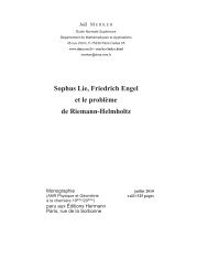
Fig. 1. Un arbre, son processus de contour <strong>et</strong> son processus des hauteurs.<br />
Nous sommes maintenant en mesure de définir les <strong>arbres</strong> de Galton-Watson. Si A est un arbre<br />
planaire <strong>et</strong> u ∈ A, on note τ u A = {v ∈ U : uv ∈ A} le sous-arbre de A issu de u. Soit µ une loi<br />
de reproduction critique ou sous-critique, ce qui signifie que ∑ k≥1 kµ(k) ≤ 1. Alors il existe une<br />
unique mesure de probabilité Π µ sur A vérifiant les deux propriétés suivantes :<br />
• Π µ (k ∅ (A) = k) = µ(k) pour tout k ≥ 0,<br />
• si µ(k) > 0, sous la mesure Π µ (· | k ∅ (A) = k), les sous <strong>arbres</strong> τ 1 A,...,τ k A sont<br />
indépendants <strong>et</strong> de loi Π µ .<br />
La mesure Π µ est par définition la loi d’un arbre de Galton-Watson de loi de reproduction µ. La<br />
deuxième propriété est une propriété de régénération. Les <strong>arbres</strong> de Galton-Watson sont ainsi<br />
les seuls <strong>arbres</strong> discr<strong>et</strong>s régénératifs. Pour p ≥ 1 <strong>et</strong> A ∈ A, on pose<br />
A p = A ∩ {u ∈ U : |u| ≤ p}.<br />
Soit p ≥ 1, soit T ∈ A tel que H(T) = p <strong>et</strong> tel que v 1 ≺ ... ≺ v m est la liste des somm<strong>et</strong>s de T à<br />
la génération p énumérés dans l’ordre lexicographique. On a alors plus généralement la propriété<br />
de régénération suivante :<br />
• si Π µ (A p = T) > 0, sous la mesure Π µ (· | A p = T), les sous <strong>arbres</strong> τ v1 A,... ,τ vm A sont<br />
indépendants <strong>et</strong> de loi Π µ .<br />
Terminons c<strong>et</strong>te sous-partie en présentant un lien entre les <strong>arbres</strong> de Galton-Watson <strong>et</strong> les<br />
marches aléatoires (voir par exemple [41]). Si µ est une loi de reproduction, on définit une mesure<br />
ν sur {−1,0,1,...} par la formule<br />
ν(k) = µ(k + 1), k ≥ −1.<br />
8
On peut alors montrer qu’il existe une marche aléatoire (X n ) n≥0 de loi de sauts ν telle que sous<br />
Π µ , presque sûrement, pour tout n ∈ {1,... ,#A − 1},<br />
{<br />
}<br />
H n = # j ∈ {1,... ,n} : X j = inf X k .<br />
j≤k≤n<br />
1.1.2. Arbres continus aléatoires. En vue d’étudier la structure limite de certains <strong>arbres</strong><br />
discr<strong>et</strong>s aléatoires, Aldous a introduit la notion d’arbre continu aléatoire.<br />
L’ensemble des <strong>arbres</strong> continus que nous considérerons est l’ensemble des <strong>arbres</strong> réels compacts<br />
enracinés. Un arbre réel est un espace métrique (T ,d) tel que pour chaque couple de points<br />
(σ 1 ,σ 2 ) de T , il existe un unique arc noté [[σ 1 ,σ 2 ]] reliant σ 1 à σ 2 , c<strong>et</strong> arc étant isométrique à un<br />
segment. Dans la suite, nous ne considérerons que des <strong>arbres</strong> réels compacts <strong>et</strong> enracinés, c’està-dire<br />
ayant un point ρ distingué, que nous appellerons la racine. Deux <strong>arbres</strong> réels compacts <strong>et</strong><br />
enracinés T <strong>et</strong> T ′ de racines respectives ρ <strong>et</strong> ρ ′ sont dits isométriques s’il existe une isométrie<br />
φ de T sur T ′ telle que φ(ρ) = ρ ′ . Nous noterons T l’ensemble des classes d’isométrie d’<strong>arbres</strong><br />
réels compacts enracinés.<br />
L’espace T est muni de la distance de Gromov-HausdorffGH définie de la façon suivante :<br />
si T <strong>et</strong> T ′ sont deux <strong>arbres</strong> réels compacts de racines respectives ρ <strong>et</strong> ρ ′ , alors<br />
GH(T , T ′ ) = inf { δ Haus (ϕ(T ),ϕ ′ (T ′ )) ∨ δ(ϕ(ρ),ϕ ′ (ρ ′ )) } ,<br />
où l’infimum est pris sur tous les plongements isométriques ϕ : T → E <strong>et</strong> ϕ ′ : T ′ → E dans un<br />
même espace métrique (E,δ). On rappelle que si (E,δ) est un espace métrique, on note δ Haus<br />
la distance de Hausdorff définie sur l’ensemble des sous-ensembles compacts de E.<br />
On peut donner une définition équivalente de la distance de Gromov-Hausdorff. Pour ce<br />
faire, il nous faut introduire la notion de correspondance entre deux espaces métriques. Une<br />
correspondance entre deux espaces métriques (E,δ) <strong>et</strong> (E ′ ,δ ′ ) est un sous-ensemble R de E ×E ′<br />
tel que pour tout x ∈ E (respectivement tout x ′ ∈ E ′ ), il existe x ′ ∈ E ′ (respectivement x ∈ E)<br />
tel que (x,x ′ ) ∈ R. La distorsion de la correspondance R est alors définie par<br />
dis(R) = sup { |δ(x,y) − δ ′ (x ′ ,y ′ )| : (x,x ′ ),(y,y ′ ) ∈ R } .<br />
Si T <strong>et</strong> T ′ sont deux <strong>arbres</strong> réels compacts de racines respectives ρ <strong>et</strong> ρ ′ , on note C(T , T ′ )<br />
l’ensemble des correspondances entre T <strong>et</strong> T ′ . On a alors<br />
GH(T , T ′ ) = 1 2 inf { dis(R) : R ∈ C(T , T ′ ),(ρ,ρ ′ ) ∈ R } .<br />
Evans, Pitman & Winter [24] ont montré que l’espace (T,GH) est un espace polonais.<br />
On peut construire un arbre réel par un codage similaire au codage d’un arbre planaire par<br />
son processus de contour. Plus précisément, si f : [0,+∞) → [0,+∞) est une fonction continue<br />
à support compact telle que f(0) = 0, on peut construire l’arbre réel compact codé par f de la<br />
façon suivante. Soit d f la pseudo-distance sur R + donnée par la relation<br />
d f (s,t) = f(s) + f(t) − 2 inf<br />
u∈[s,t] f(u),<br />
avec 0 ≤ s ≤ t. On peut alors définir une relation d’équivalence sur R + en posant s ∼ t si<br />
d f (s,t) = 0. L’arbre codé par f est alors l’espace quotient<br />
T f = [0,+∞)/ ∼<br />
muni de la distance d f <strong>et</strong> enraciné en la classe d’équivalence de 0. Pour tout s ∈ [0,+∞), on<br />
notera ṡ la classe d’équivalence de s. Ainsi ṡ est un somm<strong>et</strong> de T f à distance f(s) de la racine.<br />
9
Remarquons qu’un arbre planaire peut-être interprété comme une union de segments de<br />
longueur 1 de la façon suivante. Soit A ∈ A. On note (ǫ u ,u ∈ A \ {∅}) la base canonique de<br />
R A\{∅} . On définit une famille (l u ,u ∈ A \ {∅}) d’éléments de R A\{∅} par l u = 0 si |u| = 1, <strong>et</strong><br />
par récurrence l u = lǔ + ǫǔ si |u| ≥ 2. On pose alors<br />
T A =<br />
⋃<br />
[l u ,l u + ǫ u ].<br />
u∈A\{∅}<br />
On munit T A de la distance d A de sorte que pour tout couple de points (x,y) de T A , la distance<br />
d A (x,y) est la longueur du plus court chemin entre x <strong>et</strong> y, <strong>et</strong> l’on enracine T A en 0. Ainsi<br />
(T A ,d A ) est un arbre réel compact enraciné. Par ailleurs, notons C le processus de contour de<br />
A. On vérifie que l’arbre réel T A coïncide avec l’arbre réel T C à isométrie près. Remarquons<br />
que l’arbre planaire A ne peut être reconstruit à partir de l’arbre réel T A . En eff<strong>et</strong>, il n’y a pas<br />
d’ordre entre les enfants d’un même individu dans T A .<br />
Un premier exemple d’arbre continu aléatoire est le CRT d’Aldous [3], [4], [5]. Le CRT<br />
est défini comme l’arbre codé par √ 2e, où e = (e(t),0 ≤ t ≤ 1) est l’excursion brownienne<br />
normalisée. Si T est un arbre réel muni de la distance d, <strong>et</strong> si r > 0, alors on note rT l’arbre<br />
T muni de la distance rd. On peut alors énoncer un premier résultat de convergence dû à<br />
Aldous. Soit (A n ) n≥1 une suite d’<strong>arbres</strong> <strong>planaires</strong> aléatoires telle que chaque A n est uniformément<br />
distribué sur l’ensemble des <strong>arbres</strong> <strong>planaires</strong> à n somm<strong>et</strong>s. Alors<br />
n −1/2 T An<br />
(loi)<br />
−→<br />
n→∞ T√ 2e .<br />
Plus généralement, si µ est une loi de reproduction critique <strong>et</strong> de variance σ 2 finie, alors la loi<br />
de l’arbre réel n −1/2 T A sous Π µ (· | #A = n) converge au sens de la convergence étroite des<br />
mesures sur T vers la loi de l’arbre réel T 2e/σ quand n → ∞.<br />
1.1.3. Arbres de Lévy. Les <strong>arbres</strong> de Lévy, introduits par Duquesne & Le Gall [22],<br />
sont des analogues continus des <strong>arbres</strong> de Galton-Watson, au sens où un arbre de Lévy est un<br />
arbre continu aléatoire qui décrit la généalogie d’un processus de branchement à espace d’états<br />
continu.<br />
Soit Y = (Y t ,t ≥ 0) un processus de branchement à espace d’états continu s’éteignant<br />
presque sûrement, de mécanisme de branchement ψ, <strong>et</strong> soit X un processus de Lévy d’exposant<br />
de Laplace ψ. Duquesne & Le Gall ont montré que l’on peut définir un processus H = (H t ,t ≥ 0)<br />
par la convergence en probabilité suivante, pour tout t ≥ 0,<br />
1<br />
H t = lim<br />
ε→0 ε<br />
∫ t<br />
0½{X s≤inf s≤u≤t X u+ε} ds.<br />
Informellement, H t mesure la taille de l’ensemble {s ∈ [0,t] : X s = inf s≤u≤t X u }. Le processus H<br />
est appelé processus des hauteurs du processus Y par analogie avec le modèle discr<strong>et</strong>. Par ailleurs,<br />
notons I t = inf s∈[0,t] X s pour t ≥ 0, <strong>et</strong> N la mesure des excursions du processus (X t − I t ,t ≥ 0).<br />
Le processus H peut être défini sous N, <strong>et</strong> adm<strong>et</strong> sous N une modification continue. L’arbre<br />
de Lévy associé à H est alors l’arbre codé par H sous la mesure N <strong>et</strong> l’on note Θ ψ la “loi” de<br />
l’arbre T H sous N.<br />
Les <strong>arbres</strong> stables forment une classe importante d’<strong>arbres</strong> de Lévy. Ils sont associés aux<br />
mécanismes de branchement ψ(u) = u α pour 1 < α ≤ 2. Duquesne & Le Gall ont calculé la<br />
dimension de Hausdorff d’un arbre stable [22] <strong>et</strong> ont obtenu des résultats précis concernant la<br />
mesure de Hausdorff d’un arbre stable [23]. Par ailleurs, Miermont [46], [47] <strong>et</strong> Haas & Miermont<br />
[27] ont utilisé la structure des <strong>arbres</strong> stables pour étudier les processus de fragmentation stables.<br />
10
Enfin, les <strong>arbres</strong> de Lévy apparaissent comme les seules limites possibles pour des suites<br />
d’<strong>arbres</strong> de Galton-Watson convenablement changés d’échelle. Nous renvoyons le lecteur aux<br />
theorèmes 2.2.1 <strong>et</strong> 2.2.3 pour des énoncés précis.<br />
1.2. Arbres continus régénératifs<br />
L’obj<strong>et</strong> de c<strong>et</strong>te partie est de présenter le chapitre 2 de ce travail de thèse, qui est la version<br />
d’un article [53] soumis pour publication. Il s’agit de caractériser les <strong>arbres</strong> de Lévy par une<br />
propriété de régénération.<br />
Introduisons pour cela quelques notations. Si (T ,d) est un arbre réel compact enraciné en ρ,<br />
on note H(T ) sa hauteur c’est-à-dire<br />
H(T ) = max {d(ρ,σ) : σ ∈ T } .<br />
De plus, pour t,h > 0, on définit Z T (t,t + h) comme le nombre de sous-<strong>arbres</strong> de T issus du<br />
niveau t <strong>et</strong> de hauteur strictement supérieure à h. Duquesne & Le Gall [22] ont montré que la<br />
mesure Θ ψ vérifie la propriété de régénération suivante :<br />
(R) pour t,h > 0 <strong>et</strong> p ∈ N, sous la mesure Θ ψ (· | H(T ) > t) <strong>et</strong> conditionnellement à<br />
l’événement {Z T (t,t + h) = p}, les p sous-<strong>arbres</strong> de T issus du niveau t <strong>et</strong> de hauteur<br />
strictement supérieure à h sont indépendants <strong>et</strong> de loi Θ ψ (· | H(T ) > h).<br />
La propriété (R) est l’analogue pour des <strong>arbres</strong> continus de la propriété de régénération des<br />
<strong>arbres</strong> de Galton-Watson. Nous avons montré que c<strong>et</strong>te propriété caractérise les “lois” des <strong>arbres</strong><br />
de Lévy parmi les mesures infinies sur T.<br />
Théorème 1.2.1. Soit Θ une mesure infinie sur (T,GH) telle que Θ(H(T ) = 0) = 0 <strong>et</strong><br />
0 < Θ(H(T ) > t) < +∞ pour tout t > 0, <strong>et</strong> satisfaisant la propriété (R). Alors il existe un<br />
processus de branchement à espace d’états continu s’éteignant presque sûrement, de mécanisme<br />
de branchement ψ, tel que Θ = Θ ψ .<br />
L’idée principale de la preuve du théorème 1.2.1 est d’approcher les <strong>arbres</strong> régénératifs par<br />
des <strong>arbres</strong> de Galton-Watson. C<strong>et</strong>te idée repose sur un procédé de discrétisation des <strong>arbres</strong> réels<br />
que nous allons décrire brièvement.<br />
On se donne ε > 0, n ≥ 1 <strong>et</strong> un arbre réel T ∈ T de hauteur H(T ) vérifiant (n + 1)ε <<br />
H(T ) ≤ (n + 2)ε. Pour chaque k ∈ {0,1,... ,n}, on note σ1 k,... ,σk m k<br />
les somm<strong>et</strong>s de T à la<br />
génération kε (c’est-à-dire à distance kε de la racine) dont sont issus les sous-<strong>arbres</strong> de T au<br />
dessus du niveau kε <strong>et</strong> de hauteur strictement supérieure à ε. Chaque somm<strong>et</strong> σi<br />
k+1 appartient à<br />
un sous-arbre issu d’un élément σj k i<br />
de l’ensemble {σl k : 1 ≤ l ≤ m k }. On dit alors que l’individu<br />
σi k+1 est issu de σj k i<br />
. Une difficulté provient du fait que l’ordre entre les individus σi k+1<br />
1<br />
,... ,σi k+1<br />
l j<br />
issus d’un même parent σj k n’est pas défini. En ordonnant uniformément ces individus, on peut<br />
construire un arbre planaire A ε (T ) rendant compte de la généalogie dans l’arbre réel T de la<br />
collection de points {σi k : 1 ≤ i ≤ m k, 1 ≤ k ≤ n}.<br />
La propriété de régénération (R) nous assure alors que si T est distribué selon la mesure<br />
de probabilité Θ(· | (n + 1)ε < H(T ) ≤ (n + 2)ε), l’arbre planaire A ε (T ) est un arbre de<br />
Galton-Watson conditionné à avoir une hauteur égale à n.<br />
Dans ce travail, nous nous sommes également intéressés aux mesures de probabilité sur T<br />
vérifiant la propriété de régénération (R).<br />
11
Théorème 1.2.2. Soit Θ une mesure de probabilité sur (T,GH) telle que Θ(H(T ) = 0) = 0<br />
<strong>et</strong> 0 < Θ(H(T ) > t) pour tout t > 0, <strong>et</strong> satisfaisant la propriété (R). Alors il existe a > 0 <strong>et</strong> µ,<br />
une mesure de probabilité critique ou sous-critique sur Z + \ {1} tels que Θ est la loi de l’arbre<br />
généalogique d’un processus de branchement en temps continu, à espace d’états discr<strong>et</strong>, de loi de<br />
reproduction µ <strong>et</strong> de taux de branchement a.<br />
1.3. Arbres spatiaux aléatoires<br />
1.3.1. Arbres de Galton-Watson spatiaux. Un arbre spatial discr<strong>et</strong> est un couple<br />
(A,U) où A ∈ A <strong>et</strong> U = (U v ,v ∈ A) est une application de A dans R. On note Ω l’ensemble des<br />
<strong>arbres</strong> spatiaux discr<strong>et</strong>s.<br />
Rappelons que l’on peut coder un arbre planaire par son processus de contour C. De même,<br />
on peut définir le processus de contour spatial d’un arbre spatial discr<strong>et</strong> (A,U) en posant pour<br />
tout t ∈ [0,2(#A − 1)] entier, V (t) = U v où v est le somm<strong>et</strong> visité par C au temps t, puis on<br />
interpole linéairement V sur l’intervalle [0,2(#A − 1)]. Le couple de processus (C,V ) code alors<br />
l’arbre spatial (A,U).<br />
Soit µ une loi de reproduction <strong>et</strong> soit γ une mesure de probabilité sur R. Construisons à<br />
présent sur l’ensemble Ω la loi d’un arbre de Galton-Watson spatial de loi de reproduction µ <strong>et</strong><br />
dont les déplacements spatiaux sont régis par γ. Soit A ∈ A <strong>et</strong> soit x ∈ R. On définit la mesure<br />
R x (A,dU) sur R A de la façon suivante. Considérons une suite (Y u ,u ∈ U) de variables aléatoires<br />
indépendantes <strong>et</strong> de loi γ. On pose U ∅ = x <strong>et</strong> pour tout v ∈ A \ {∅},<br />
U v = ∑<br />
Y v ′,<br />
v ′ ∈]∅,v]<br />
où ]∅,v] est l’ensemble des ancêtres de v privé de la racine ∅ (noter que v ∈]∅,v]). La mesure<br />
R x (A,dU) est alors la loi de (U v ,v ∈ A). Posons<br />
P x (dAdU) = Π µ (dA)R x (A,dU).<br />
On dit que la mesure P x est la loi d’un arbre de Galton-Watson spatial issu de x, de loi de<br />
reproduction µ <strong>et</strong> de loi de déplacement spatial γ.<br />
1.3.2. Arbre brownien <strong>et</strong> serpent brownien. L’arbre brownien est un arbre réel spatial<br />
aléatoire. Un arbre réel spatial est un couple (T ,Y ) où T est un arbre réel compact <strong>et</strong> enraciné<br />
<strong>et</strong> Y = (Y σ ,σ ∈ T ) est une application continue de T dans R. Deux <strong>arbres</strong> réels spatiaux (T ,Y )<br />
<strong>et</strong> (T ′ ,Y ′ ) sont dits isométriques si T <strong>et</strong> T ′ sont isométriques <strong>et</strong> si pour tout σ ∈ T ,<br />
Y ′ φ(σ) = Y σ,<br />
où φ est une isométrie de T sur T ′ telle que φ(ρ) = ρ ′ . On notera T sp l’ensemble des classes<br />
d’isométrie d’<strong>arbres</strong> réels spatiaux.<br />
Rappelons que C(T , T ′ ) est l’ensemble des correspondances entre T <strong>et</strong> T ′ <strong>et</strong> que si R ∈<br />
C(T , T ′ ), alors on note dis(R) la distorsion de R. On définit sur T sp une distancesp par la<br />
formule suivante :<br />
(<br />
sp (T ,Y ),(T ′ ,Y ′ ) ) {<br />
}<br />
= 1 2 inf dis(R) + sup |Y σ − Y σ ′ ′| : R ∈ C(T , T ′ ),(ρ,ρ ′ ) ∈ R .<br />
(σ,σ ′ )∈R<br />
On vérifie alors que l’espace T sp muni de la distancesp est un espace polonais.<br />
12
Nous pouvons maintenant définir l’arbre brownien. Si T ∈ T <strong>et</strong> x ∈ R, on note Q x (T ,dY ) la<br />
loi du processus gaussien (Y σ ,σ ∈ T ) caractérisé par<br />
• E(Y σ ) = x,<br />
• Cov(Y σ ,Y σ ′) = d(ρ,σ ∧ σ ′ ),<br />
où σ ∧ σ ′ est le plus proche ancêtre commun à σ <strong>et</strong> σ ′ , c’est-à-dire le somm<strong>et</strong> de T vérifiant<br />
la relation [[ρ,σ ∧ σ ′ ]] = [[ρ,σ]] ∩ [[ρ,σ ′ ]] (sous une hypothèse faible sur T toujours réalisée dans<br />
la suite, (Y σ ,σ ∈ T ) a une modification continue). Notons n la loi de l’excursion brownienne<br />
normalisée. On définit une mesure de probabilité N x (dT dY ) sur T sp en posant<br />
∫<br />
∫ ∫<br />
N x (dT dY )F(T ,Y ) = n(de) Q x (T e ,dY )F(T e ,Y ).<br />
La mesure N x est la loi de l’arbre brownien issu de x 1 .<br />
Le serpent brownien, introduit par Le Gall, est un obj<strong>et</strong> intimement lié à l’arbre brownien.<br />
Nous renvoyons le lecteur à [37] pour une présentation détaillée du serpent brownien <strong>et</strong> de<br />
certaines de ses applications. Le serpent brownien est un processus de Markov à valeurs dans<br />
l’espace des trajectoires arrêtées<br />
W = ⋃<br />
C([0,t], R).<br />
t∈R +<br />
Pour tout w ∈ W, on pose ζ w = t si w ∈ C([0,t], R). Autrement dit, ζ w représente le temps<br />
de vie de la trajectoire w. De plus, on note ŵ = w(ζ w ) le point terminal de w. On définit une<br />
distance d W sur W de la façon suivante :<br />
d W (w,w ′ ) = sup<br />
t≥0<br />
∣<br />
∣w(t ∧ ζ w ) − w ′ (t ∧ ζ w ′) ∣ + |ζ w − ζ w ′|.<br />
On peut alors montrer que l’espace W muni de la distance d W est un espace polonais.<br />
Construisons à présent le serpent brownien “conditionnellement à son temps de vie”. Pour<br />
cela, on se donne une fonction continue f : [0,1] −→ [0,+∞) telle que f(0) = 0, <strong>et</strong> l’on pose<br />
pour tous 0 ≤ s ≤ s ′ ≤ 1,<br />
m(s,s ′ ) = inf<br />
u∈[s,s ′ ] f(u).<br />
Soit x ∈ R. Il existe alors un processus de Markov inhomogène (W s ,0 ≤ s ≤ 1) à valeurs dans W<br />
tel que W 0 = x presque sûrement, <strong>et</strong> dont le noyau de transition est caractérisé par la description<br />
suivante : pour tous 0 ≤ s ≤ s ′ ≤ 1,<br />
• W s ′(t) = W s (t) pour tout t ≤ m(s,s ′ ), presque sûrement,<br />
• (W s ′(m(s,s ′ ) + t) − W s (m(s,s ′ )),0 ≤ t ≤ f(s ′ ) − m(s,s ′ )) est indépendant de W s <strong>et</strong><br />
suit la loi d’un mouvement brownien partant de 0.<br />
On note θ f x la loi du processus (W s ,s ≥ 0) <strong>et</strong> l’on pose,<br />
N x (dζ dW) = n(dζ)θ ζ x(dW).<br />
Le serpent brownien est alors le processus canonique ((ζ s ,0 ≤ s ≤ 1),(W s ,0 ≤ s ≤ 1)) de<br />
l’espace C([0,1], R + ) × C([0,1], W) muni de la mesure de probabilité N x .<br />
Remarquons que l’on peut définir sous N x un processus Y = (Y σ ,σ ∈ T ζ ) en posant pour<br />
tout s ∈ [0,1] tel que σ = ṡ,<br />
Y σ = Ŵs.<br />
1 Les notations n <strong>et</strong> Nx introduites ici n’ont pas les mêmes significations que dans le chapitre 3.<br />
13
Rappelons que si s ∈ [0,1], alors ṡ est la classe d’équivalence de s pour la relation d’équivalence<br />
définie par ζ. En outre, on voit que la loi de (T ζ ,Y ) est la mesure N x .<br />
Une mesure aléatoire est naturellement associée à l’arbre brownien. Il s’agit de la mesure Z<br />
sur R définie par<br />
∫ 1<br />
∫ 1 )<br />
〈Z,ϕ〉 = ϕ(Yṡ)ds = ϕ<br />
(Ŵs ds.<br />
0<br />
C<strong>et</strong>te mesure aléatoire est appelée Integrated Super-Brownian Excursion (ISE). La mesure ISE<br />
en grande dimension intervient dans divers résultats asymptotiques de modèles de mécanique<br />
statistique (voir par exemple [18], [28], [29]).<br />
Enfin, l’arbre brownien apparaît comme limite de suites d’<strong>arbres</strong> spatiaux discr<strong>et</strong>s convenablement<br />
renormalisés. Plus précisément, Janson & Marckert [31] ont montré le résultat suivant.<br />
Soit µ une loi de reproduction critique telle qu’il existe η > 0 satisfaisant<br />
∑<br />
e ηk µ(k) < +∞.<br />
k≥0<br />
Soit γ une mesure de probabilité sur R, de moyenne nulle <strong>et</strong> vérifiant la condition de moments<br />
suivante : quand y → +∞,<br />
γ ({|u| > y}) = o ( y −4) .<br />
Les lois µ <strong>et</strong> γ ont donc des variances finies <strong>et</strong> l’on pose Var(µ) = ϑ 2 µ <strong>et</strong> Var(γ) = ϑ 2 γ. Rappelons<br />
que si A est un arbre planaire, on note C le processus de contour de A <strong>et</strong> V le processus de<br />
contour spatial de A. Alors, pour tout x ∈ R, la loi sous la mesure P x (· | #A = n) de<br />
⎛<br />
⎝(<br />
ϑµ<br />
2<br />
)<br />
C(2nt)<br />
√ n<br />
0≤t≤1<br />
,<br />
(<br />
(<br />
1 ϑµ<br />
ϑ γ 2<br />
0<br />
) )<br />
1/2<br />
V (2nt)<br />
n 1/4<br />
0≤t≤1<br />
converge quand n → ∞ vers la loi sous la mesure de probabilité N 0 du couple<br />
(<br />
)<br />
(ζ s ,0 ≤ s ≤ 1),(Ŵs,0 ≤ s ≤ 1) .<br />
1.4. Arbre brownien conditionné<br />
Nous présentons dans c<strong>et</strong>te partie le chapitre 3 de ce travail de thèse, qui est une version d’un<br />
article [42] écrit en collaboration avec Jean-François Le Gall <strong>et</strong> paru aux annales de l’institut<br />
Henri Poincaré. Il s’agit de définir l’arbre brownien issu de 0 conditionné à rester positif.<br />
Pour (T ,Y ) ∈ T sp , on note X T ,Y = {Y σ : σ ∈ T }. On cherche donc à conditionner l’arbre<br />
brownien issu de 0 par l’événement {X T ,Y ⊂ [0,+∞)}. Ce <strong>conditionnement</strong> est un <strong>conditionnement</strong><br />
dégénéré car<br />
N 0 (X T ,Y ⊂ [0,+∞)) = 0.<br />
En revanche, pour tout ε > 0, on a<br />
N 0 (X T ,Y ⊂ (−ε,+∞)) > 0.<br />
L’idée est donc de construire la loi de l’arbre brownien conditionné à rester positif comme la<br />
limite en un certain sens des mesures N 0 (dT dY | X T ,Y ⊂ (−ε,+∞)).<br />
Théorème 1.4.1. On a<br />
N 0 (X T ,Y ⊂ (−ε, ∞))<br />
lim<br />
ε↓0 ε 4 = 2<br />
21 .<br />
⎞<br />
⎠<br />
14
De plus, il existe une mesure N 0 sur l’espace T sp telle que<br />
lim<br />
ε↓0<br />
N 0 (dT dY | X T ,Y ⊂ (−ε, ∞)) = N 0 (dT dY ),<br />
au sens de la convergence étroite des mesures sur T sp .<br />
Le deuxième théorème principal de ce travail donne une représentation explicite de l’arbre réel<br />
spatial de loi N 0 au moyen d’une transformation de l’arbre brownien analogue à la transformation<br />
de Vervaat du pont brownien.<br />
Rappelons brièvement en quoi consiste la transformation de Vervaat du pont brownien. Soit<br />
(B t ,t ∈ [0,1]) un pont brownien sur [0,1]. Il est connu que presque sûrement, il existe un unique<br />
instant t ∗ ∈ [0,1] tel que<br />
B t∗ = min<br />
t∈[0,1] B t.<br />
On définit un processus B ∗ = (B ∗ t ,t ∈ [0,1]) par la transformation<br />
B ∗ t = B {t∗+t} − B t∗ ,<br />
où {t ∗ + t} est la partie fractionnaire de t ∗ + t. Vervaat [52] a montré que la loi du processus B ∗<br />
est alors la loi n de l’excursion brownienne normalisée.<br />
La transformation que nous effectuons sur les <strong>arbres</strong> réels spatiaux est une opération de<br />
“réenracinement au minimum”. Présentons tout d’abord en quoi consiste le réenracinement d’un<br />
arbre réel spatial en l’un de ses somm<strong>et</strong>s. Si (T ,Y ) ∈ T sp <strong>et</strong> σ ∈ T , on définit l’arbre réenraciné<br />
(T [σ] ,Y [σ] ) de la façon suivante. L’arbre T [σ] est l’arbre T , mais sa racine est le somm<strong>et</strong> σ <strong>et</strong><br />
non plus ρ. Puis on translate les positions spatiales en posant pour tout σ ′ ∈ T ,<br />
Y [σ]<br />
σ ′ = Y σ ′ − Y σ .<br />
Par ailleurs, on montre (voir la proposition 3.2.5) que sous la mesure N 0 , il existe presque<br />
sûrement un unique somm<strong>et</strong> σ ∗ ∈ T tel que<br />
Y σ∗ = min {Y σ : σ ∈ T }.<br />
On est alors en mesure d’énoncer le deuxième théorème principal de ce travail.<br />
Théorème 1.4.2. La mesure N 0 est la loi sous N 0 de l’arbre réenraciné (T [σ∗] ,Y [σ∗] ).<br />
Le point de départ de la preuve de ce théorème est une propriété d’invariance de l’opération<br />
de réenracinement sous N 0 . Marckert & Mokkadem [45] (voir aussi le théorème 3.2.3) ont montré<br />
que pour toute fonction mesurable positive sur T sp <strong>et</strong> pour tout s ∈ [0,1], on a<br />
(<br />
N 0<br />
(F T [ṡ] ,Y [ṡ])) = N 0 (F(T ,Y )) .<br />
Les théorèmes 1.4.1 <strong>et</strong> 1.4.2 peuvent être exprimés en termes du serpent brownien. Tout<br />
d’abord, notons que la proposition 3.2.5 nous assure que N 0 presque sûrement, il existe un<br />
unique s ∗ ∈ [0,1] tel que<br />
}<br />
Ŵ s∗ = min{Ŵs : s ∈ [0,1] = min {W s (t) : t ∈ [0,ζ s ], s ∈ [0,1]} .<br />
De plus, pour tout s ∈ [0,1], on pose<br />
ζ [s]<br />
r = ζ s + ζ {s+r} − 2 inf<br />
[s,{s+r}] ζ,<br />
Ŵ [s]<br />
r<br />
= Ŵ{s+r} − Ŵs.<br />
15
On définit ensuite W [s] à partir de Ŵ [s] de la façon suivante : pour tout r ∈ [0,1] <strong>et</strong> tout<br />
t ∈ [0,ζ r [s] ],<br />
[s]<br />
(t) = Ŵ n<br />
o.<br />
W [s]<br />
r<br />
sup<br />
u≤r:ζ u [s] =t<br />
Notons X = {Ŵs : s ∈ [0,1]}. On a alors l’existence d’une mesure N 0 sur C(R + , R + )×C(R + , W)<br />
telle que<br />
N 0 (dζ dW | X ⊂ (−ε,+∞)) −→<br />
ε↓0<br />
N 0 (dζ dW),<br />
au sens de la convergence étroite des mesures sur C(R + , R + ) × C(R + , W). De plus N 0 est la loi<br />
sous N 0 du serpent réenraciné (ζ [s∗] ,W [s∗] ).<br />
De même que précédemment, on définit sous N 0 un processus Y = (Y σ ,σ ∈ T ζ ) en posant<br />
pour tout s ∈ [0,1] tel que σ = ṡ,<br />
Y σ = Ŵs.<br />
Alors la loi de (T ζ ,Y ) sous N 0 est la mesure N 0 .<br />
Une des motivations de ce travail était d’exhiber un arbre aléatoire qui serait une limite<br />
possible de suites d’<strong>arbres</strong> discr<strong>et</strong>s conditionnés à rester positifs, <strong>et</strong> convenablement renormalisés.<br />
Le Gall [39] a montré le résultat suivant. Notons, pour (A,U) ∈ Ω,<br />
U = min{U v : v ∈ A \ {∅}}.<br />
Supposons que les lois µ <strong>et</strong> γ vérifient les mêmes hypothèses que celles du résultat de Janson<br />
& Marckert <strong>et</strong> que la loi γ est symétrique. Alors pour tout x > 0, la loi sous la mesure de<br />
probabilité P x (· | #A = n + 1,U > 0) de<br />
⎛<br />
⎝(<br />
ϑµ<br />
2<br />
)<br />
C(2nt)<br />
√ n<br />
0≤t≤1<br />
,<br />
(<br />
(<br />
1 ϑµ<br />
ϑ γ 2<br />
) )<br />
1/2<br />
V (2nt)<br />
n 1/4<br />
0≤t≤1<br />
converge quand n → ∞ vers la loi sous la mesure de probabilité N 0 du couple<br />
(<br />
)<br />
(ζ s ,0 ≤ s ≤ 1),(Ŵs,0 ≤ s ≤ 1) .<br />
Dans ce travail nous nous sommes également intéressés au <strong>conditionnement</strong> de l’arbre brownien<br />
ayant une hauteur fixée. Pour h > 0, on note n h la loi de l’excursion brownienne de hauteur<br />
h. On définit une mesure de probabilité N h x (dT dY ) en posant pour x ∈ R,<br />
∫<br />
∫ ∫<br />
N h x(dT dY )F(T ,Y ) = n h (de) Q x (T e ,dY )F(T e ,Y ).<br />
Rappelons que si f : [0,+∞) −→ [0,+∞) est une fonction continue à support compact telle que<br />
f(0) = 0, on dit que f est de hauteur h si<br />
max f(s) = h.<br />
s∈[0,+∞)<br />
Remarquons que si f est de hauteur h, alors H(T f ) = h. On dit que N h x est la loi de l’arbre<br />
brownien de hauteur h issu de x.<br />
Théorème 1.4.3. Pour tout h > 0, il existe une mesure de probabilité N h 0 sur T sp telle que<br />
lim<br />
ε→0 Nh 0(dT dY | X T ,Y ⊂ (−ε,+∞)) = N h 0(dT dY ),<br />
au sens de la convergence étroite des mesures sur T sp .<br />
⎞<br />
⎠<br />
16
Décrivons l’arbre réel spatial de loi N h 0 . Tout d’abord, on peut montrer que Nh 0 presque<br />
sûrement, il existe un unique somm<strong>et</strong> σ ∈ T tel que<br />
d(ρ,σ) = h.<br />
Pour tout t ∈ [0,h], soit σ t l’unique point de l’arc [[ρ,σ]] tel que d(ρ,σ t ) = t. On définit alors un<br />
processus (R h t ,0 ≤ t ≤ h) par la relation,<br />
R h t = Y σ t<br />
, t ∈ [0,h].<br />
On montre que la loi du processus (Rt h ,0 ≤ t ≤ h) est absolument continue par rapport à la loi<br />
de (β t ,0 ≤ t ≤ h) où β est un processus de Bessel de dimension 9. Nous renvoyons à la partie<br />
3.4 pour l’expression explicite de la densité de la loi de (Rt h ,0 ≤ t ≤ h) par rapport à la loi du<br />
processus de Bessel (β t ,0 ≤ t ≤ h). De plus, on montre que le processus (Rt∧h h ,t ≥ 0) converge<br />
en loi vers (β t ,t ≥ 0) quand h → ∞.<br />
Par ailleurs, notons (T i ,i ∈ I) la famille des sous-<strong>arbres</strong> de T issus de l’arc [[ρ,σ]]. Soit σ i le<br />
point de [[ρ,σ]] dont est issu le sous-arbre T i . On pose<br />
On définit alors une mesure ponctuelle M par<br />
d i = d(ρ,σ i ).<br />
M = ∑ i∈I<br />
δ (di ,T i ).<br />
Puis, si l > 0, on note n
1.5. Arbres spatiaux <strong>et</strong> <strong>cartes</strong> <strong>planaires</strong><br />
1.5.1. Lois de Boltzmann sur les <strong>cartes</strong> <strong>planaires</strong>. Une carte planaire M est un plongement<br />
d’un graphe connexe G dans la sphère bidimensionnelle S 2 , c’est à dire un “dessin” de<br />
G dans S 2 tel que les arêtes ne se rencontrent qu’au niveau des somm<strong>et</strong>s. Une face de M est<br />
une composante connexe de S 2 \ M, <strong>et</strong> son degré est le nombre d’arêtes de M incluses dans sa<br />
ferm<strong>et</strong>ure. Une carte planaire est dite bipartie si chacune de ses faces est de degré pair. Une<br />
carte planaire est une 2κ-angulation si chacune de ses faces est de degré 2κ.<br />
Si M est une carte planaire, on notera respectivement V M , E M <strong>et</strong> F M l’ensemble des somm<strong>et</strong>s,<br />
des arêtes <strong>et</strong> des faces de M. L’ensemble V M est muni de la distance de graphe, c’est-à-dire que la<br />
distance entre deux somm<strong>et</strong>s de M est la longueur du plus court chemin entre ces deux somm<strong>et</strong>s.<br />
Une carte planaire pointée est un couple (M,τ) où M est une carte planaire <strong>et</strong> τ est un<br />
somm<strong>et</strong> distingué de M. Une carte planaire enracinée est un couple (M,⃗e ) où M est une carte<br />
planaire <strong>et</strong> ⃗e est une arête orientée de M. On appelle somm<strong>et</strong> racine le point dont est issue l’arête<br />
orientée ⃗e. Une carte planaire enracinée <strong>et</strong> pointée est un tripl<strong>et</strong> (M,τ,e) où (M,τ) est une carte<br />
planaire pointée <strong>et</strong> e est une arête non orientée de M. Remarquons que l’on peut interpréter une<br />
carte enracinée (M,⃗e ) comme une carte enracinée <strong>et</strong> pointée en conservant l’arête non-orientée<br />
e <strong>et</strong> en choisissant le somm<strong>et</strong> racine comme point distingué.<br />
On identifie deux <strong>cartes</strong> <strong>planaires</strong> pointées (respectivement enracinées, enracincées <strong>et</strong> pointées)<br />
M <strong>et</strong> M ′ s’il existe un homéomorphisme de S 2 préservant l’orientation, qui envoie M sur M ′ <strong>et</strong><br />
qui préserve le point distingué (respectivement l’arête orientée, le point distingué <strong>et</strong> l’arête nonorientée).<br />
On note respectivement M p , M r <strong>et</strong> M r,p , l’ensemble des <strong>cartes</strong> <strong>planaires</strong> pointées,<br />
enracinées <strong>et</strong> enracinées <strong>et</strong> pointées après l’identification précédente.<br />
On définit à partir d’une suite q = (q i ) i≥1 de poids positifs telle que q i > 0 pour au moins un<br />
indice i ≥ 2, une mesure de Boltzmann sur l’ensemble M r,p de la façon suivante. Pour M ∈ M r,p ,<br />
on pose<br />
W q (M) = ∏<br />
q deg(f)/2 ,<br />
f∈F M<br />
où deg(f) est le degré de la face f. Si la suite q vérifie<br />
Z q =<br />
∑<br />
W q (M) < ∞,<br />
M∈M r,p<br />
on dit que q est admissible <strong>et</strong> l’on définit la distribution de Boltzmann B r,p<br />
q sur l’ensemble M r,p<br />
par<br />
B r,p<br />
q (M) = W q(M)<br />
.<br />
Z q<br />
De plus, on définit pour M ∈ M r<br />
Z q (r) = ∑ ∏<br />
q deg(f)/2 .<br />
f∈F M<br />
La condition Z q < ∞ implique que Z q<br />
(r)<br />
sur l’ensemble M r par<br />
M∈M r<br />
< ∞. Alors on définit la distribution de Boltzmann B r q<br />
B r q(M) = W q(M)<br />
Z q<br />
(r) .<br />
18
On pose N(k) = ( 2k−1<br />
k−1<br />
)<br />
pour k ≥ 1. Pour tout suite q de poids comme précédemment on<br />
définit<br />
f q (x) = ∑ k≥0<br />
N(k + 1)q k+1 x k , x ≥ 0,<br />
<strong>et</strong> l’on note R q le rayon de convergence de la série entière f q . D’après la proposition 1 dans [43],<br />
la suite q est admissible si <strong>et</strong> seulement si l’équation<br />
(1.5.1) f q (x) = 1 − 1 x , x > 0,<br />
adm<strong>et</strong> au moins une solution. Dans ce cas Z q est la solution de (1.5.1) vérifiant<br />
On dit que la suite q est régulière si<br />
Z 2 q f ′ q (Z q) ≤ 1.<br />
Z 2 q f ′ q (Z q) = 1.<br />
Si de plus Z q < R q on dit que q est critique régulière.<br />
Présentons finalement un cas particulier de mesure de Boltzmann ne chargeant que l’ensemble<br />
des 2κ-angulations. Soit κ ≥ 2. On pose<br />
α κ =<br />
(κ − 1)κ−1<br />
κ κ N(κ) .<br />
Soit q κ la suite de poids définie par q κ = α κ <strong>et</strong> q i = 0 pour tout i ∈ N \ {κ}. D’après la partie<br />
1.5 dans [43], la suite q κ est critique régulière <strong>et</strong><br />
Z qκ =<br />
κ<br />
κ − 1 .<br />
Pour tout n ≥ 1, notons respectivement U n κ <strong>et</strong> U n κ la mesure uniforme sur l’ensemble des 2κangulations<br />
enracinées <strong>et</strong> pointées <strong>et</strong> la mesure uniforme sur l’ensemble des 2κ-angulations enracinées.<br />
On voit alors que<br />
B r,p<br />
q κ<br />
(· | #F M = n) = U n κ,<br />
B r q κ<br />
(· | #F M = n) = U n κ .<br />
1.5.2. Loi de Boltzmann sur l’ensemble des mobiles. Dans c<strong>et</strong>te partie, on interprétera<br />
les <strong>arbres</strong> spatiaux comme des <strong>arbres</strong> spatiaux à deux types en déclarant que les somm<strong>et</strong>s<br />
des générations paires sont de type 0 <strong>et</strong> les somm<strong>et</strong>s des générations impaires sont de type 1.<br />
Pour (A,U) ∈ A, on pose<br />
A 0<br />
A 1<br />
= {u ∈ A : |u| est pair},<br />
= {u ∈ A : |u| est impair}.<br />
Un mobile (enraciné) est un arbre spatial à deux types (A,U) tel que les propriétés suivantes<br />
sont vérifiées :<br />
(a) U v = Uˇv pour tout v ∈ A 1 .<br />
(b) Soit v ∈ A 1 tel que k v (A) = k ≥ 1. On note v (0) = ˇv le père de v <strong>et</strong> v (j) = vj pour tout<br />
j ∈ {1,... ,k}. Alors pour tout j ∈ {0,... ,k},<br />
où par convention v (k+1) = v (0) .<br />
U v(j+1) ≥ U v(j) − 1,<br />
19
Si de plus U v ≥ 1 pour tout v ∈ A, alors (A,U) est un mobile bien étiqu<strong>et</strong>é.<br />
Construisons à présent une loi de Galton-Watson sur l’ensemble des mobiles de la façon<br />
expliquée dans [43]. Soit q une suite de poids critique régulière. Notons µ q 0 la loi géométrique<br />
de paramètre f q (Z q ) c’est-à-dire la mesure sur {0,1,2,...} définie pour k ≥ 0 par<br />
<strong>et</strong> µ q 1<br />
µ q 0 (k) = f q(Z q ) k<br />
Z q<br />
,<br />
la mesure sur {0,1,2,...} définie pour k ≥ 0 par<br />
µ q 1 (k) = Zk qN(k + 1)q k+1<br />
.<br />
f q (Z q )<br />
On pose µ q = (µ q 0 ,µq 1 ). On définit une mesure de probabilité P µ q sur l’ensemble des <strong>arbres</strong><br />
<strong>planaires</strong> par la formule suivante : pour t ∈ A,<br />
P µ q(t) = ∏ u∈t 0 µ q 0 (k u(t)) ∏ u∈t 1 µ q 1 (k u(t)).<br />
Pour tout k ≥ 1 on note ν0 k la mesure de Dirac en 0 ∈ Rk <strong>et</strong> ν1 k la mesure uniforme sur<br />
l’ensemble A k défini par<br />
{<br />
}<br />
A k = (x 1 ,...,x k ) ∈ Z k : x 1 ≥ −1,x 2 − x 1 ≥ −1,... ,x k − x k−1 ≥ −1, −x k ≥ −1 .<br />
La mesure ν1 k est alors la loi du vecteur (X 1,X 1 + X 2 ,...,X 1 + ... + X k ) où (X 1 ,...,X k+1 ) est<br />
uniformément distribué sur l’ensemble B k defini par<br />
{<br />
}<br />
B k = (x 1 ,...,x k+1 ) ∈ {−1,0,1,2,...} k+1 : x 1 + ... + x k+1 = 0 .<br />
Soit A ∈ A. On définit une mesure de probabilité R ν,1 (A,dU) sur R A de la façon suivante.<br />
Soit (Y u ,u ∈ A) une suite de vecteurs aléatoires indépendants telle que pour u ∈ A vérifiant<br />
k u (A) = k, le vecteur Y u = (Y u1 ,... ,Y uk ) est de loi ν0 k si u ∈ A0 <strong>et</strong> de loi ν1 k si u ∈ A1 . On<br />
définit U ∅ = 1 <strong>et</strong> pour tout v ∈ A \ {∅},<br />
U v = 1 + ∑<br />
Y u ,<br />
u∈]∅,v]<br />
où ]∅,v] représente l’ensemble des ancêtres de v privé de la racine ∅. La mesure R ν,1 (A,dU)<br />
est alors la loi de (U v ,v ∈ A).<br />
Soit P µ,ν,1 la mesure de probabilité définie par<br />
P µ,ν,1 (dAdU) = P µ (dA)R ν,1 (A,dU).<br />
On vérifie facilement que la mesure P µ,ν,1 ne charge que l’ensemble des mobiles (A,U) tels que<br />
U ∅ = 1.<br />
1.5.3. La bijection de Bouttier, di Francesco & Guitter. Bouttier, di Francesco &<br />
Guitter [11] ont établi une bijection entre l’ensemble des mobiles bien étiqu<strong>et</strong>és <strong>et</strong> l’ensemble<br />
des <strong>cartes</strong> biparties enracinées. C<strong>et</strong>te bijection est une généralisation de la bijection construite<br />
par Schaeffer [51] entre les <strong>arbres</strong> bien étiqu<strong>et</strong>és <strong>et</strong> les quadrangulations enracinées (voir aussi<br />
[15] pour une étude antérieure de c<strong>et</strong>te bijection).<br />
Présentons dans un premier temps une version de la bijection de Bouttier, di Francesco &<br />
Guitter entre l’ensemble des mobiles <strong>et</strong> l’ensemble des <strong>cartes</strong> biparties enracinées <strong>et</strong> pointées.<br />
Soit (A,U) un mobile tel que U ∅ = 1. On pose ξ = #A−1 <strong>et</strong> l’on définit une suite w 0 ,w 1 ,... ,w ξ<br />
20
de somm<strong>et</strong>s de A 0 de telle sorte que pour tout k ∈ {0,1,... ,ξ}, le somm<strong>et</strong> w k est le somm<strong>et</strong><br />
visité par le contour de A au temps 2k. De plus on définit un mobile bien étiqu<strong>et</strong>é (A,U + ) par<br />
la relation pour v ∈ A<br />
U + v = U v − min{U w : w ∈ A} + 1.<br />
Notons que<br />
min { U + w : w ∈ A} = 1.<br />
Supposons maintenant que l’arbre planaire A est dessiné dans le plan <strong>et</strong> ajoutons un somm<strong>et</strong><br />
∂. On associe au mobile (A,U) une carte planaire dont l’ensemble des somm<strong>et</strong>s est<br />
A 0 ∪ {∂},<br />
<strong>et</strong> dont les arêtes sont obtenues par le procédé suivant :<br />
• si U + w k<br />
= 1, on trace une arête entre w k <strong>et</strong> ∂,<br />
• si U + w k<br />
≥ 2, on trace une arête entre w k <strong>et</strong> le premier somm<strong>et</strong> parmi w k+1 ,...,w ξ−1 ,<br />
w 0 ,...,w k−1 dont l’étiqu<strong>et</strong>te est U + w k<br />
− 1.<br />
La condition (b) de la définition d’un mobile garantit que si U + w k<br />
≥ 2, alors il existe un somm<strong>et</strong><br />
parmi w k+1 ,...,w ξ−1 ,w 0 ,...,w k−1 dont l’étiqu<strong>et</strong>te est U + w k<br />
− 1. La carte planaire ainsi obtenue<br />
est une carte bipartie que l’on pointe en ∂ <strong>et</strong> que l’on enracine en l’arête obtenue pour k = 0<br />
dans la construction précédente.<br />
Bouttier, di Francesco & Guitter [11] ont montré que la construction précédente fournit une<br />
bijection Ψ r,p entre l’ensemble des mobiles (A,U) tels que U ∅ = 1 <strong>et</strong> l’ensemble des <strong>cartes</strong><br />
biparties enracinées <strong>et</strong> pointées.<br />
On remarque que si (A,U) est un mobile bien étiqu<strong>et</strong>é tel que U ∅ = 1 alors U + v = U v pour<br />
tout v ∈ A. En particulier U + ∅ = 1. On en déduit que l’arête distinguée de la carte Ψ r,p((A,U))<br />
contient le point ∂. On peut ainsi indentifier Ψ r,p ((A,U)) à une carte enracinée. Cela implique<br />
que la bijection Ψ r,p induit une bijection Ψ r entre l’ensemble des mobiles bien étiqu<strong>et</strong>és (A,U)<br />
tels que U ∅ = 1 <strong>et</strong> l’ensemble M r (voir la figure 2).<br />
La bijection Ψ r vérifie les deux propriétés suivantes : soit (A,U) un mobile tel que U ∅ = 1<br />
<strong>et</strong> soit M = Ψ((A,U)),<br />
• pour tout k ≥ 1, l’ensemble {f ∈ F M : deg(f) = 2k} est en bijection avec l’ensemble<br />
{v ∈ A 1 : k v (A) = k},<br />
• pour tout l ≥ 1, l’ensemble {a ∈ V M : d(∂,a) = l} est en bijection avec l’ensemble<br />
{v ∈ A 0 : U v = l}.<br />
Enfin signalons la propriété suivante (voir la proposition 10 dans [43]). La distribution de<br />
Boltzmann conditionnée B r,p<br />
q (· | #F M = n) est l’image de la mesure P µ q ,ν,1(· | #A 1 = n) par<br />
l’application Ψ r,p . De plus, pour tout mobile (A,U) on définit<br />
U = min { U v : v ∈ A 0 \ {∅} } .<br />
La distribution de Boltzmann conditionnée B r q (· | #F M = n) est alors l’image de la mesure<br />
P µ q ,ν,1(· | #A 1 = n, U ≥ 1) par l’application Ψ r .<br />
21
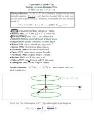
Fig. 2. Construction d’une carte bipartie enracinée à partir d’un mobile bien étiqu<strong>et</strong>é<br />
1.5.4. Un théorème limite pour les mobiles. En vue d’étudier certaines propriétés<br />
asymptotiques des grandes <strong>cartes</strong> biparties enracinées <strong>et</strong> pointées, Marckert & Miermont [43]<br />
ont établi un théorème limite pour les mobiles.<br />
Avant d’énoncer ce résultat, rappelons que si (A,U) est un arbre spatial, on note C son<br />
processus de contour <strong>et</strong> V son processus de contour spatial. De plus, pour toute suite de poids<br />
critique régulière q, on pose<br />
ρ q = 2 + Zqf 3 q(Z ′′ q ).<br />
Marckert & Miermont [43] ont montré le théorème suivant : si q est une suite critique régulière,<br />
alors la loi sous la mesure P µ q ,ν,1(· | #A 1 = n) de<br />
( (αq ( )<br />
C(2(#A − 1)t) βq V (2(#A − 1)t)<br />
n<br />
)0≤t≤1<br />
1/2 ,<br />
n<br />
)0≤t≤1<br />
1/4<br />
converge (au sens de la convergence étroite des mesures sur C([0,1], R 2 ) quand n → ∞ vers la<br />
loi de (ζ,Ŵ) sous la mesure N 0, où les constantes α q <strong>et</strong> β q sont définies par les formules<br />
√<br />
ρq (Z q − 1)<br />
α q =<br />
,<br />
4<br />
( ) 9(Zq − 1) 1/4<br />
β q =<br />
.<br />
4ρ q<br />
Ce résultat est un cas particulier du théorème 11 dans [43] qui traite d’<strong>arbres</strong> de Galton-Watson<br />
spatiaux à deux types plus généraux. Signalons que dans le cas particulier q = q κ les constantes<br />
apparaissant dans le résultat précédent sont données par<br />
α qκ = 1 ( ) κ 1/2<br />
,<br />
4 κ − 1<br />
β qκ =<br />
(<br />
9<br />
4κ(κ − 1)<br />
) 1/4<br />
.<br />
22
1.6. Résultats asymptotiques pour de grandes <strong>cartes</strong> biparties enracinées<br />
aléatoires<br />
C<strong>et</strong>te partie récapitule les résultats du chapitre 4 de ce travail de thèse, dans lequel nous nous<br />
intéressons à certaines propriétés asymptotiques de grandes <strong>cartes</strong> <strong>planaires</strong> biparties enracinées<br />
aléatoires.<br />
Introduisons au préalable quelques notations. Soit M ∈ M r . On note o le somm<strong>et</strong> racine de<br />
M c’est-à-dire le somm<strong>et</strong> dont est issue l’arête racine. Soit<br />
R M = max {d(o,a) : a ∈ V M } ,<br />
le rayon de la carte M. Le profil de M est la mesure de probabilité sur {0,1,2,...} définie par<br />
λ M (k) = #{a ∈ V M : d(o,a) = k}<br />
, k ≥ 0.<br />
#V M<br />
Si M a n faces, on définit enfin le profil de M changé d’échelle par la relation suivante,<br />
où A est un borélien de R + .<br />
λ (n)<br />
M (A) = λ M<br />
(<br />
n 1/4 A<br />
)<br />
,<br />
Théorème 1.6.1. Soit q une suite de poids critique régulière.<br />
(i) La loi de n −1/4 R M sous la mesure de probabilité B r q(· | #F M = n) converge quand<br />
n → ∞ vers la loi sous la mesure N 0 de la variable aléatoire<br />
(<br />
)<br />
1<br />
sup Ŵ(s) − inf Ŵ(s) .<br />
β q 0≤s≤1<br />
0≤s≤1<br />
(ii) La loi de la mesure aléatoire λ (n)<br />
M sous la mesure de probabilité Br q (· | #F M = n)<br />
converge quand n → ∞ vers la loi sous la mesure N 0 de la mesure aléatoire I définie<br />
par<br />
〈I,g〉 =<br />
∫ 1<br />
0<br />
( ( 1<br />
g<br />
β q<br />
Ŵ(t) −<br />
inf<br />
0≤s≤1<br />
))<br />
Ŵ(s) dt.<br />
(iii) La loi de n −1/4 d(o,a) où a est uniformément distribué sur V M , sous la mesure de<br />
probabilité B r q(· | #F M = n), converge quand n → ∞ vers la loi sous la mesure N 0 de<br />
la variable aléatoire ( )<br />
1<br />
sup Ŵ(s) .<br />
β q<br />
0≤s≤1<br />
Le théorème 1.6.1 est une généralisation des résultats obtenus par Chassaing & Schaeffer [14]<br />
qui traitent le cas particulier q = q 2 des quadrangulations (voir aussi le théorème 8.2 dans [39]).<br />
Le théorème 1.6.1 est aussi très proche du théorème 3 de [43] qui a largement motivé notre<br />
étude. La différence vient de ce que [43] considère des <strong>cartes</strong> enracinées <strong>et</strong> pointées, <strong>et</strong> étudie<br />
les distances à partir du somm<strong>et</strong> distingué <strong>et</strong> non du somm<strong>et</strong> racine comme nous le faisons ici.<br />
Signalons que dans le cas q = q 2 , la constante qui apparaît dans le théorème 1.6.1 vaut<br />
( )<br />
1 8 1/4<br />
= .<br />
β q2 9<br />
La preuve du théorème 1.6.1 repose sur un théorème limite pour les mobiles bien étiqu<strong>et</strong>és.<br />
23
Théorème 1.6.2. Soit q une suite de poids critique régulière. La loi sous la mesure de<br />
probabilité P µ q ,ν,1(· | #A 1 = n, U ≥ 1) de<br />
( (αq ( )<br />
C(2(#A − 1)t) βq V (2(#A − 1)t)<br />
n<br />
)0≤t≤1<br />
1/2 ,<br />
n<br />
)0≤t≤1<br />
1/4<br />
converge (au sens de la convergence étroite des mesures sur C([0,1], R) 2 ) quand n → ∞ vers la<br />
loi de (ζ,Ŵ) sous la mesure N 0.<br />
Le théorème 1.6.1 se déduit du théorème 1.6.2 en utilisant les propriétés vérifiées par la<br />
bijection de Bouttier, di Francesco & Guitter. En particulier on observe que la loi de R M sous<br />
la mesure B r q coïncide avec la loi de la variable aléatoire<br />
sup {U v : v ∈ A}<br />
sous la mesure P µ q ,ν,1(· | #A 1 = n,U ≥ 1). Or le théorème 1.6.2 implique que la loi sous la<br />
mesure P µ q ,ν,1(· | #A 1 = n, U ≥ 1) de<br />
1<br />
n<br />
supU 1/4 v<br />
v∈A<br />
converge quand n → ∞ vers la loi sous N 0 de la variable aléatoire<br />
1<br />
sup Ŵ s ,<br />
β q 0≤s≤1<br />
c’est-à-dire d’après le théorème 1.4.2, la loi sous N 0 de la variable aléatoire<br />
(<br />
)<br />
1<br />
sup Ŵ s − inf Ŵ s .<br />
β q 0≤s≤1<br />
0≤s≤1<br />
La preuve du théorème 1.6.2 s’articule de manière analogue à la preuve du théorème 2.2 dans<br />
[39]. En particulier, une étape cruciale est le calcul d’estimations de la probabilité<br />
P µ q ,ν,1<br />
(<br />
U ≥ 1 | #A 1 = n ) .<br />
Proposition 1.6.3. Il existe des constantes γ > 0 <strong>et</strong> ˜γ > 0 telles que pour tout n suffisamment<br />
grand,<br />
γ<br />
n ≤ P (<br />
µ q ,ν,1 U ≥ 1 | #A 1 = n ) ≤ ˜γ n .<br />
C<strong>et</strong>te proposition nous perm<strong>et</strong> d’obtenir des résultats asymptotiques concernant les points<br />
de disconnection dans les grandes 2κ-angulations enracinées uniformes.<br />
Soit M une carte planaire <strong>et</strong> soit σ 0 un somm<strong>et</strong> de M. Soit σ ∈ V M \ {σ 0 }. On note S σ 0,σ<br />
M<br />
l’ensemble des somm<strong>et</strong>s a de M tel que tout chemin allant de σ à a passe par σ 0 . On dit que σ 0<br />
est un point de disconnection de M s’il existe σ ∈ V M \ {σ 0 } tel que S σ 0,σ<br />
M ≠ {σ 0} <strong>et</strong> l’on note<br />
D M l’ensemble des points de disconnection de la carte M.<br />
Soit (A,U) un mobile <strong>et</strong> soit v ∈ A 0 . Rappelons que τ v A = {w ∈ U,vw ∈ A}. Supposons que<br />
(τ v A) 0 ≠ {v} <strong>et</strong> que la condition suivante est satisfaite :<br />
inf { U vw : w ∈ (τ v A) 0 \ {∅} } > U v .<br />
On remarque alors que dans la construction de la carte M = Ψ r,p ((A,U)) l’ensemble S v,τ<br />
M<br />
est en<br />
bijection avec (τ v A) 0 (où l’on a noté τ le point distingué de la carte enracinée <strong>et</strong> pointée M).<br />
Le somm<strong>et</strong> v est donc un point de disconnection de M.<br />
24
Rappelons que U n κ <strong>et</strong> U n κ désignent respectivement la mesure uniforme sur l’ensemble des<br />
2κ-angulations enracinées <strong>et</strong> pointées à n faces <strong>et</strong> la mesure uniforme sur l’ensemble des 2κangulations<br />
enracinées à n faces. On montre alors le résultat suivant en utilisant la remarque<br />
précédente <strong>et</strong> la proposition 1.6.3.<br />
Théorème 1.6.4. Pour tout ε > 0,<br />
lim<br />
n→∞ Un κ<br />
(<br />
∃ σ 0 ∈ D M : σ 0 ≠ τ, n 1/2−ε ≤ #S σ 0,τ<br />
M ≤ 2n1/2−ε) = 1.<br />
Remarquons que si M est une 2κ-angulation à n faces alors d’après la formule d’Euler<br />
#V M = n(κ − 1) + 2.<br />
On déduit alors du théorème 1.6.4 le résultat suivant.<br />
Théorème 1.6.5. Pour tout ε > 0,<br />
lim<br />
n→∞ U n κ<br />
(<br />
∃ σ 0 ∈ D M : ∃ σ ∈ V M \ {σ 0 }, n 1/2−ε ≤ #S σ 0,σ<br />
M ≤ 2n1/2−ε) = 1.<br />
25
CHAPITRE 2<br />
Regenerative real trees<br />
2.1. Introduction<br />
Galton-Watson trees are well known to be characterized among all random discr<strong>et</strong>e trees by<br />
a regenerative property. More precisely, if µ is a probability measure on Z + , the law Π µ of the<br />
Galton-Watson tree with offspring distribution µ is uniquely d<strong>et</strong>ermined by the following two<br />
conditions : under the probability measure Π µ ,<br />
(i) the ancestor has p children with probability µ(p),<br />
(ii) if µ(p) > 0, then conditionally on the event that the ancestor has p children, the p subtrees<br />
which describe the genealogy of the descendants of these children are independent<br />
and distributed according to Π µ .<br />
The aim of this work is to study σ-finite measures satisfying an analogue of this property on<br />
the space of equivalence classes of rooted compact R-trees.<br />
An R-tree is a m<strong>et</strong>ric space (T ,d) such that for any two points σ 1 and σ 2 in T there is a<br />
unique arc with endpoints σ 1 and σ 2 , and furthermore this arc is isom<strong>et</strong>ric to a compact interval<br />
of the real line. We denote this arc by [[σ 1 ,σ 2 ]]. In this work, all R-trees are supposed to be<br />
compact. A rooted R-tree is an R-tree with a distinguished vertex called the root. Say that two<br />
rooted R-trees are equivalent if there is a root-preserving isom<strong>et</strong>ry that maps one onto the other.<br />
It was noted in [24] that the s<strong>et</strong> T of all equivalence classes of rooted compact R-trees equipped<br />
with the pointed Gromov-Hausdorff distanceGH (see e.g. Chapter 7 in [12]) is a Polish space.<br />
Hence it is legitimate to consider random variables with values in T, that is, random R-trees.<br />
A particularly important example is the CRT, which was introduced by Aldous [3], [5] with a<br />
different formalism. Striking applications of the concept of random R-trees can be found in the<br />
recent papers [24] and [25].<br />
L<strong>et</strong> T be an R-tree. We write H(T ) for the height of the R-tree T , that is, the maximal<br />
distance from the root to a vertex of T . For every t ≥ 0, we denote by T ≤t the s<strong>et</strong> of all vertices<br />
of T which are at distance at most t from the root, and by T >t the s<strong>et</strong> of all vertices which are<br />
at distance greater than t from the root. To each connected component of T >t there corresponds<br />
a “subtree” of T above level t (see section 2.2.2.3 for a more precise definition). For every h > 0,<br />
we define Z(t,t+h)(T ) as the number of subtrees of T above level t with height greater than h.<br />
L<strong>et</strong> Θ be a σ-finite measure on T such that 0 < Θ(H(T ) > t) < ∞ for every t > 0 and<br />
Θ(H(T ) = 0) = 0. We say that Θ satisfies the regenerative property (R) if the following holds :<br />
(R) for every t,h > 0 and p ∈ N, under the probability measure Θ(· | H(T ) > t) and<br />
conditionally on the event {Z(t,t + h) = p}, the p subtrees of T above level t with<br />
height greater than h are independent and distributed according to the probability<br />
measure Θ(· | H(T ) > h).<br />
This is a natural analogue of the regenerative property stated above for Galton-Watson trees.<br />
Beware that, unlike the discr<strong>et</strong>e case, there is no natural order on the subtrees above a given<br />
27
level. So, the preceding property should be understood in the sense that the unordered collection<br />
of the p subtrees in consideration is distributed as the unordered collection of p independent<br />
copies of Θ(· | H(T ) > h).<br />
Property (R) is known to be satisfied by a wide class of infinite measures on T, namely the<br />
“laws” of Lévy trees. Lévy trees have been introduced by T. Duquesne and J.F. Le Gall in<br />
[22]. Their precise definition is recalled in section 2.2.3, but l<strong>et</strong> us immediately give an informal<br />
presentation.<br />
L<strong>et</strong> Y be a critical or subcritical continuous-state branching process. The distribution of Y<br />
is characterized by its branching mechanism function ψ. Assume that Y becomes extinct a.s.,<br />
which is equivalent to the condition ∫ ∞<br />
1<br />
ψ(u) −1 du < ∞. The ψ-Lévy tree is a random variable<br />
taking values in (T,GH), which describes the genealogy of a population evolving according to<br />
Y and starting with infinitesimally small mass. More precisely, the “law” of the Lévy tree is<br />
defined in [22] as a σ-finite measure on the space (T,GH), such that 0 < Θ ψ (H(T ) > t) < ∞<br />
for every t > 0. As a consequence of Theorem 4.2 of [22], the measure Θ ψ satisfies Property<br />
(R). In the special case ψ(u) = u α , 1 < α ≤ 2 corresponding to the so-called stable trees, this<br />
was used by Miermont [46], [47] to introduce and to study certain fragmentation processes.<br />
In the present work we describe all σ-finite measures on T that satisfy Property (R). We<br />
show that the only infinite measures satisfying Property (R) are the measures Θ ψ associated<br />
with Lévy trees. On the other hand, if Θ is a finite measure satisfying Property (R), we can<br />
obviously restrict our attention to the case Θ(T) = 1 and we obtain that Θ must be the law of<br />
the genealogical tree associated with a continuous-time discr<strong>et</strong>e-state branching process.<br />
Theorem 2.1.1. L<strong>et</strong> Θ be an infinite measure on (T,GH) such that Θ(H(T ) = 0) = 0 and<br />
0 < Θ(H(T ) > t) < +∞ for every t > 0. Assume that Θ satisfies Property (R). Then, there<br />
exists a continuous-state branching process, whose branching mechanism is denoted by ψ, which<br />
becomes extinct almost surely, such that Θ = Θ ψ .<br />
Theorem 2.1.2. L<strong>et</strong> Θ be a probability measure on (T,GH) such that Θ(H(T ) = 0) = 0<br />
and 0 < Θ(H(T ) > t) for every t > 0. Assume that Θ satisfies Property (R). Then there<br />
exists a > 0 and a critical or subcritical probability measure γ on Z + \{1} such that Θ is the<br />
law of the genealogical tree for a discr<strong>et</strong>e-space continuous-time branching process with offspring<br />
distribution γ, where branchings occur at rate a.<br />
In other words, Θ in Theorem 2.1.2 can be described in the following way : there exists a real<br />
random variable J such that under Θ :<br />
(i) J is distributed according to the exponential distribution with param<strong>et</strong>er a and there<br />
exists σ J ∈ T such that T ≤J = [[ρ,σ J ]],<br />
(ii) the number of subtrees above level J is distributed according to γ and is independent<br />
of J,<br />
(iii) for every p ≥ 2, conditionally on J and given the event that the number of subtrees<br />
above level J is equal to p, these p subtrees are independent and distributed according<br />
to Θ.<br />
Theorem 2.1.1 is proved in section 2.3, after some preliminary results have been established in<br />
section 2.2. A key idea of the proof is to use the regenerative property to embed discr<strong>et</strong>e Galton-<br />
Watson trees in our random real trees (Lemma 2.3.3). A technical difficulty comes from the<br />
fact that real trees are not ordered whereas Galton-Watson trees are usually defined as random<br />
ordered discr<strong>et</strong>e trees (cf subsection 2.2.2.4 below). To overcome this difficulty, we assign a<br />
28
andom ordering to the discr<strong>et</strong>e trees embedded in real trees. Another major ingredient of the<br />
proof of Theorem 2.1.1 is the construction of a “local time” L t at every level t of a random real<br />
tree governed by Θ. The local time process is then shown to be a continuous-state branching<br />
process with branching mechanism ψ, which makes it possible to identify Θ with Θ ψ . Theorem<br />
2.1.2 is proved in section 2.4. Several arguments are similar to the proof of Theorem 2.1.1, so<br />
that we have skipped some d<strong>et</strong>ails.<br />
2.2. Preliminaries<br />
In this section, we recall some basic facts about branching processes, R-trees and Lévy trees.<br />
2.2.1. Branching processes.<br />
2.2.1.1. Continuous-state branching processes. A (continuous-time) continuous-state branching<br />
process (in short a CSBP) is a Markov process Y = (Y t ,t ≥ 0) with values in the positive<br />
half-line [0,+∞), with a Feller semigroup (Q t ,t ≥ 0) satisfying the following branching property :<br />
for every t ≥ 0 and x,x ′ ≥ 0,<br />
Q t (x, ·) ∗ Q t (x ′ , ·) = Q t (x + x ′ , ·).<br />
Informally, this means that the union of two independent populations started respectively at x<br />
and x ′ will evolve like a single population started at x + x ′ .<br />
We will consider only the critical or subcritical case, meaning that for every t ≥ 0 and x ≥ 0,<br />
∫<br />
yQ t (x,dy) ≤ x.<br />
[0,+∞)<br />
Then, if we exclude the trivial case where Q t (x, ·) = δ 0 for every t > 0 and x ≥ 0, the Laplace<br />
functional of the semigroup can be written in the following form : for every λ ≥ 0,<br />
∫<br />
e −λy Q t (x,dy) = exp(−xu(t,λ)),<br />
[0,+∞)<br />
where the function (u(t,λ),t ≥ 0,λ ≥ 0) is d<strong>et</strong>ermined by the differential equation<br />
du(t,λ)<br />
= −ψ(u(t,λ)), u(0,λ) = λ,<br />
dt<br />
and ψ : R + −→ R + is of the form<br />
∫<br />
(2.2.1) ψ(u) = αu + βu 2 + (e −ur − 1 + ur)π(dr),<br />
(0,+∞)<br />
where α,β ≥ 0 and π is a σ-finite measure on (0,+∞) such that ∫ (0,+∞) (r ∧ r2 )π(dr) < ∞. The<br />
process Y is called the ψ-continuous-state branching process (in short the ψ-CSBP).<br />
Continuous-state branching processes may also be obtained as weak limits of rescaled Galton-<br />
Watson processes. We recall that an offspring distribution is a probability measure on Z + . An<br />
offspring distribution µ is said to be critical if ∑ i≥0 iµ(i) = 1 and subcritical if ∑ i≥0<br />
iµ(i) < 1.<br />
L<strong>et</strong> us state a result that can be derived from [26] and [30].<br />
Theorem 2.2.1. L<strong>et</strong> (µ n ) n≥1 be a sequence of offspring distributions. For every n ≥ 1, denote<br />
by X n a Galton-Watson process with offspring distribution µ n , started at X n 0 = n. L<strong>et</strong> (m n) n≥1<br />
be a nondecreasing sequence of positive integers converging to infinity. We define a sequence of<br />
processes (Y n ) n≥1 by s<strong>et</strong>ting, for every t ≥ 0 and n ≥ 1,<br />
Y n<br />
t = n −1 X n [m nt] .<br />
29
Assume that, for every t ≥ 0, the sequence (Y n<br />
t ) n≥1 converges in distribution to Y t where Y =<br />
(Y t ,t ≥ 0) is an almost surely finite process such that P(Y δ > 0) > 0 for some δ > 0. Then, Y<br />
is a continuous-state branching process and the sequence of processes (Y n ) n≥1 converges to Y in<br />
distribution in the Skorokhod space D(R + ).<br />
Proof : It follows from the proof of Theorem 1 of [30] that Y is a CSBP. Then, thanks to<br />
Theorem 2 of [30], there exists a sequence of offspring distributions (ν n ) n≥1 and a nondecreasing<br />
sequence of positive integers (c n ) n≥1 such that we can construct for every n ≥ 1 a Galton-Watson<br />
process Z n started at c n and with offspring distribution ν n satisfying<br />
where the symbol<br />
(<br />
c −1<br />
n Zn [nt] ,t ≥ 0 )<br />
d<br />
−→<br />
n→∞ (Y t,t ≥ 0),<br />
d<br />
−→ indicates convergence in distribution in D(R + ).<br />
L<strong>et</strong> (m nk ) k≥1 be a strictly increasing subsequence of (m n ) n≥1 . For n ≥ 1, we s<strong>et</strong> B n = X n k<br />
and b n = n k if n = m nk for some k ≥ 1, and we s<strong>et</strong> B n = Z n and b n = c n if there is no<br />
k ≥ 1 such that n = m nk . Then, for every t ≥ 0, (b −1<br />
n Bn [nt] ) n≥1 converges in distribution to Y t .<br />
Applying Theorem 4.1 of [26], we obtain that<br />
( )<br />
b −1<br />
n Bn [nt] ,t ≥ 0 d<br />
−→ (Y t,t ≥ 0).<br />
n→∞<br />
In particular, we have,<br />
( )<br />
(2.2.2)<br />
Y n k d<br />
t ,t ≥ 0 −→ (Y t,t ≥ 0).<br />
k→∞<br />
As (2.2.2) holds for every strictly increasing subsequence of (m n ) n≥1 , we obtain the desired<br />
result.<br />
□<br />
2.2.1.2. Discr<strong>et</strong>e-state branching processes. A (continuous-time) discr<strong>et</strong>e-state branching process<br />
(in short DSBP) is a continuous-time Markov chain Y = (Y t ,t ≥ 0) with values in Z + whose<br />
transition probabilities (P t (i,j),t ≥ 0) i≥0,j≥0 satisfy the following branching property : for every<br />
i ∈ Z + , t ≥ 0 and |s| ≤ 1,<br />
⎛ ⎞i<br />
∞∑<br />
∞∑<br />
P t (i,j)s j = ⎝ P t (1,j)s j ⎠ .<br />
j=0<br />
We exclude the trivial case where P t (i,i) = 1 for every t ≥ 0 and i ∈ Z + . Then, there exist<br />
a > 0 and an offspring distribution γ with γ(1) = 0 such that the generator of Y can be written<br />
of the form ⎛<br />
⎞<br />
0 0 0 0 0 ...<br />
aγ(0) −a aγ(2) aγ(3) aγ(4) ...<br />
Q =<br />
0 2aγ(0) −2a 2aγ(2) aγ(3) ...<br />
.<br />
⎜<br />
⎝ 0 0 3aγ(0) −3a 3aγ(2) ... ⎟<br />
⎠<br />
.<br />
. . .. . .. . .. . ..<br />
Furthermore, it is well known that Y becomes extinct almost surely if and only if γ is critical<br />
or subcritical. We refer the reader to [7] and [49] for more d<strong>et</strong>ails.<br />
2.2.2. D<strong>et</strong>erministic trees.<br />
j=0<br />
30
2.2.2.1. The space (T,GH) of rooted compact R-trees. We start with a basic definition.<br />
Definition 2.2.1. A m<strong>et</strong>ric space (T ,d) is an R-tree if the following two properties hold for<br />
every σ 1 ,σ 2 ∈ T .<br />
(i) There is a unique isom<strong>et</strong>ric map f σ1 ,σ 2<br />
from [0,d(σ 1 ,σ 2 )] into T such that f σ1 ,σ 2<br />
(0) = σ 1<br />
and f σ1 ,σ 2<br />
(d(σ 1 ,σ 2 )) = σ 2 .<br />
(ii) If q is a continuous injective map from [0,1] into T such that q(0) = σ 1 and q(1) = σ 2 ,<br />
we have<br />
q([0,1]) = f σ1 ,σ 2<br />
([0,d(σ 1 ,σ 2 )]).<br />
A rooted R-tree is an R-tree with a distinguished vertex ρ = ρ(T ) called the root.<br />
In what follows, R-trees will always be rooted.<br />
L<strong>et</strong> (T ,d) be an R-tree with root ρ, and σ,σ 1 ,σ 2 ∈ T . We write [[σ 1 ,σ 2 ]] for the range of the<br />
map f σ1 ,σ 2<br />
. In particular, [[ρ,σ]] is the path going from the root to σ and can be interpr<strong>et</strong>ed as<br />
the ancestral line of σ.<br />
The height H(T ) of the R-tree T is defined by H(T ) = sup{d(ρ,σ) : σ ∈ T }. In particular,<br />
if T is compact, its height H(T ) is finite.<br />
Two rooted R-trees T and T ′ are called equivalent if there is a root-preserving isom<strong>et</strong>ry that<br />
maps T onto T ′ . We denote by T the s<strong>et</strong> of all equivalence classes of rooted compact R-trees.<br />
We often abuse notation and identify a rooted compact R-tree with its equivalence class.<br />
The s<strong>et</strong> T can be equipped with the pointed Gromov-Hausdorff distance, which is defined<br />
as follows. If (E,δ) is a m<strong>et</strong>ric space, we use the notation δ Haus for the usual Hausdorff m<strong>et</strong>ric<br />
b<strong>et</strong>ween compact subs<strong>et</strong>s of E. Then, if T and T ′ are two rooted compact R-trees with respective<br />
roots ρ and ρ ′ , we define the distanceGH(T , T ′ ) as<br />
{<br />
GH(T , T ′ (<br />
) = inf δ Haus φ(T ),φ ′ (T ′ ) ) }<br />
∨ δ(φ(ρ),φ ′ (ρ ′ )) ,<br />
where the infimum is over all isom<strong>et</strong>ric embeddings φ : T −→ E and φ ′ : T ′ −→ E into a<br />
common m<strong>et</strong>ric space (E,δ). We see thatGH(T , T ′ ) only depends on the equivalence classes<br />
of T and T ′ . Furthermore, according to Theorem 2 in [24],GH defines a m<strong>et</strong>ric on T that<br />
makes it compl<strong>et</strong>e and separable. Notice thatGH(T , T ′ ) makes sense more generally if T and<br />
T ′ are pointed compact m<strong>et</strong>ric spaces (see e.g. Chapter 7 in [12]). We will use this in the proof<br />
of Lemma 2.2.2 below.<br />
We equip T with its Borel σ-field.<br />
If T ∈ T, we s<strong>et</strong> T ≤t = {σ ∈ T : d(ρ,σ) ≤ t} for every t ≥ 0. Plainly, T ≤t is an R-tree whose<br />
root is the same as the root of T . Note that the mapping T ↦−→ T ≤t from T into T is Lipschitz<br />
for the Gromov-Hausdorff m<strong>et</strong>ric.<br />
2.2.2.2. The R-tree coded by a function. We now recall a construction of rooted compact<br />
R-trees which is described in [22]. L<strong>et</strong> g : [0,+∞) −→ [0,+∞) be a continuous function with<br />
compact support satisfying g(0) = 0. We exclude the trivial case where g is identically zero. For<br />
every s,t ≥ 0, we s<strong>et</strong><br />
m g (s,t) = inf g(r)<br />
r∈[s∧t,s∨t]<br />
and<br />
d g (s,t) = g(s) + g(t) − 2m g (s,t).<br />
31
We define an equivalence relation ∼ on [0,+∞) by declaring that s ∼ t if and only if d g (s,t) = 0<br />
(or equivalently if and only if g(s) = g(t) = m g (s,t)). L<strong>et</strong> T g be the quotient space<br />
T g = [0,+∞)/ ∼ .<br />
Then, d g induces a m<strong>et</strong>ric on T g and we keep the notation d g for this m<strong>et</strong>ric. According to<br />
Theorem 2.1 of [22], the m<strong>et</strong>ric space (T g ,d g ) is a compact R-tree. By convention, its root is the<br />
equivalence class of 0 for ∼ and is denoted by ρ g .<br />
2.2.2.3. Subtrees of a tree above a fixed level. L<strong>et</strong> (T ,d) ∈ T and t > 0. Denote by T i,◦ ,i ∈ I<br />
the connected components of the open s<strong>et</strong> T >t = {σ ∈ T : d(ρ(T ),σ) > t}. L<strong>et</strong> i ∈ I. Then<br />
the ancestor of σ at level t, that is, the unique vertex on the line segment [[ρ,σ]] at distance<br />
t from ρ, must be the same for all σ ∈ T i,◦ . We denote by σ i this common ancestor and s<strong>et</strong><br />
T i = T i,◦ ∪ {σ i }. Thus T i is a compact rooted R-tree with root σ i . The trees T i ,i ∈ I are called<br />
the subtrees of T above level t. We now consider, for every h > 0,<br />
Z(t,t + h)(T ) = #{i ∈ I : H(T i ) > h}.<br />
By a compactness argument, we can easily verify that Z(t,t + h)(T ) < ∞.<br />
2.2.2.4. Discr<strong>et</strong>e trees and real trees. We start with some formalism for discr<strong>et</strong>e trees. We<br />
first introduce the s<strong>et</strong> of labels<br />
U = ⋃ n≥0<br />
N n ,<br />
where by convention N 0 = {∅}. An element of U is a sequence u = u 1 ...u n , and we s<strong>et</strong> |u| = n<br />
so that |u| represents the generation of u. In particular, |∅| = 0. If u = u 1 ...u n and v = v 1 ...v m<br />
belong to U, we write uv = u 1 ...u n v 1 ...v m for the concatenation of u and v. In particular,<br />
∅u = u∅ = u. The mapping π : U\{∅} −→ U is defined by π(u 1 ...u n ) = u 1 ... u n−1 (π(u) is<br />
the father of u). Note that π k (u) = ∅ if k = |u|.<br />
A rooted ordered tree θ is a finite subs<strong>et</strong> of U such that<br />
(i) ∅ ∈ θ,<br />
(ii) u ∈ θ\{∅} ⇒ π(u) ∈ θ,<br />
(iii) for every u ∈ θ, there exists a number k u (θ) ≥ 0 such that uj ∈ θ if and only if<br />
1 ≤ j ≤ k u (θ).<br />
We denote by A the s<strong>et</strong> of all rooted ordered trees. If θ ∈ A, we write H(θ) for the height of θ, that<br />
is H(θ) = max{|u| : u ∈ θ}. And for every u ∈ θ, we define τ u θ ∈ A by τ u θ = {v ∈ U : uv ∈ θ}.<br />
This is the tree θ shifted at u.<br />
L<strong>et</strong> us define an equivalence relation on A by s<strong>et</strong>ting θ ≡ θ ′ if and only if we can find a<br />
permutation ϕ u of the s<strong>et</strong> {1,... ,k u (θ)} for every u ∈ θ such that k u (θ) ≥ 1, in such a way that<br />
{<br />
θ ′ (<br />
= {∅} ∪ ϕ ∅ u<br />
1 ) (<br />
ϕ u 1 u<br />
2 ) ...ϕ u 1 ...u n−1 (un ) : u 1 ...u n ∈ θ, n ≥ 1}<br />
.<br />
In other words θ ≡ θ ′ if they correspond to the same unordered tree. L<strong>et</strong> A = A/ ≡ be the<br />
associated quotient space and l<strong>et</strong>Ô:A−→ A be the canonical projection. It is immediate that<br />
if θ ≡ θ ′ , then k ∅ (θ) = k ∅ (θ ′ ). So, for every ξ ∈ A, we may define k ∅ (ξ) = k ∅ (θ) where θ is any<br />
representative of ξ.<br />
L<strong>et</strong> us fix ξ ∈ A such that k ∅ (ξ) = k > 0 and choose a representative θ of ξ. We may<br />
define {ξ 1 ,... ,ξ k } = {Ô(τ 1 θ),...,Ô(τ k θ)} as the unordered family of subtrees of ξ above the<br />
32
first generation. Then, if F : A k −→ R + is any symm<strong>et</strong>ric measurable function, we have<br />
( #Ô−1 (ξ) ) −1<br />
∑<br />
F(τ 1 θ,...,τ k θ)<br />
(2.2.3)<br />
=<br />
θ∈Ô−1 (ξ)<br />
( ) −1 ( ) −1 ∑<br />
#Ô−1 (ξ 1 ) ... #Ô−1 (ξ k )<br />
θ 1 ∈Ô−1 (ξ 1 )<br />
...<br />
∑<br />
θ k ∈Ô−1 (ξ k )<br />
F(θ 1 ,...,θ k ).<br />
Note that the right-hand side of (2.2.3) is well defined since it is symm<strong>et</strong>ric in {ξ 1 ,...,ξ k }. The<br />
identity (2.2.3) is a simple combinatorial fact, whose proof is left to the reader.<br />
A marked tree is a pair T = (θ, {h u } u∈θ ) where θ ∈ A and h u ≥ 0 for every u ∈ θ. We denote<br />
by M the s<strong>et</strong> of all marked trees. We can associate with every marked tree T = (θ, {h u } u∈θ ) ∈ M,<br />
an R-tree T T in the following way. L<strong>et</strong> R θ be the vector space of all mappings from θ into R.<br />
Write (e u ,u ∈ θ) for the canonical basis of R θ . We define l ∅ = 0 and l u = ∑ |u|<br />
k=1 h π k (u)e π k (u) for<br />
u ∈ θ \ {∅}. L<strong>et</strong> us s<strong>et</strong><br />
T T =<br />
u∈θ[l ⋃ u ,l u + h u e u ].<br />
T T is a connected union of line segments in R θ . It is equipped with the distance d T such that<br />
d T (a,b) is the length of the shortest path in T T b<strong>et</strong>ween a and b, and can be rooted in ρ(T T ) = 0<br />
so that it becomes a rooted compact R-tree.<br />
If θ ∈ A, we write T θ for the R-tree T T where T = (θ, {h u } u∈θ ) with h ∅ = 0 and h u = 1<br />
for every u ∈ θ \ {∅}, and we write d θ for the associated distance. We then s<strong>et</strong> m ∅ = 0 and<br />
m u = ∑ |u|−1<br />
k=0 e π k (u) = l u + e u for every u ∈ θ \ {∅}.<br />
It is easily checked that T θ = T θ′ if θ ≡ θ ′ . Thus for every ξ ∈ A, we may write T ξ for the<br />
tree T θ where θ is any representative of ξ.<br />
We will now explain how to approximate a general tree T in T by a discr<strong>et</strong>e type tree. L<strong>et</strong><br />
ε > 0 and s<strong>et</strong> T (ε) = {T ∈ T : H(T ) > ε}. For every T in T (ε) , we can construct by induction<br />
an element ξ ε (T ) of A in the following way.<br />
• If T ∈ T (ε) satisfies H(T ) ≤ 2ε, we s<strong>et</strong> ξ ε (T ) =Ô({∅}).<br />
• L<strong>et</strong> n be a positive integer. Assume that we have defined ξ ε (T ) for every T ∈ T (ε) such<br />
that H(T ) ≤ (n + 1)ε. L<strong>et</strong> T be an R-tree such that (n + 1)ε < H(T ) ≤ (n + 2)ε. We<br />
s<strong>et</strong> k = Z(ε,2ε)(T ) and we denote by T 1 ,... , T k the k subtrees of T above level ε with<br />
height greater than ε. Then ε < H(T i ) ≤ (n + 1)ε for every i ∈ {1,... ,k}, so we can<br />
define ξ ε (T i ). L<strong>et</strong> us choose a representative θ i of ξ ε (T i ) for every i ∈ {1,... ,k}. We<br />
s<strong>et</strong><br />
ξ ε (T ) =Ô({∅} ∪ 1θ 1 ∪ ... ∪ kθ k) ,<br />
where iθ i = {iu : u ∈ θ i }. Clearly this does not depend on the choice of the representatives<br />
θ i .<br />
If r > 0 and T is a compact rooted R-tree with m<strong>et</strong>ric d, we write rT for the same tree<br />
equipped with the m<strong>et</strong>ric rd.<br />
Lemma 2.2.2. For every ε > 0 and every T ∈ T (ε) , we have<br />
( )<br />
(2.2.4) GH εT ξε (T ) , T ≤ 4ε.<br />
Proof : L<strong>et</strong> ε > 0 and T ∈ T. L<strong>et</strong> θ be any representative of ξ ε (T ). Recall the notation<br />
(m u ,u ∈ θ). We can construct a mapping φ : θ −→ T such that :<br />
33
(i) for every σ ∈ T , there exists u ∈ θ such that d(σ,φ(u)) ≤ 2ε,<br />
(ii) for every u ∈ θ, d(φ(u),ρ) = ε|u| where ρ denotes the root of T ,<br />
(iii) for every u,u ′ ∈ θ, 0 ≤ εd θ (m u ,m u ′) − d(φ(u),φ(u ′ )) ≤ 2ε.<br />
To be specific, we always take φ(∅) = ρ, which suffices for the construction if H(T ) ≤ 2ε. If<br />
(n + 1)ε < H(T ) ≤ (n + 2)ε for some n ≥ 1, we have as above<br />
θ = {∅} ∪ 1θ 1 ∪ ... ∪ kθ k ,<br />
where θ 1 ,... ,θ k are representatives of respectively ξ ε (T 1 ),... ,ξ ε (T k ), if T 1 ,... , T k are the<br />
subtrees of T above level ε with height greater than ε. With an obvious notation we define<br />
φ(ju) = φ j (u) for every j ∈ {1,... ,k} and u ∈ θ j . Properties (i)-(iii) are then easily checked by<br />
induction.<br />
L<strong>et</strong> us now s<strong>et</strong> Φ = {φ(u),u ∈ θ} and M = {m u ,u ∈ θ}. We equip Φ with the m<strong>et</strong>ric<br />
induced by d and M with the m<strong>et</strong>ric induced by εd θ . Then, Φ and M can be viewed as pointed<br />
compact m<strong>et</strong>ric spaces with respective roots ρ and 0. It is immediate thatGH(εT θ ,M) ≤ ε.<br />
Furthermore, Property (i) above implies thatGH(T ,Φ) ≤ 2ε. At last, according to Lemma 2.3<br />
in [24] and Property (iii) above, we haveGH(Φ,M) ≤ ε. Lemma 2.2.2 then follows from the<br />
triangle inequality forGH.<br />
□<br />
2.2.3. Lévy trees. Roughly speaking, a Lévy tree is a T-valued random variable which is<br />
associated with a CSBP in such a way that it describes the genealogy of a population evolving<br />
according to this CSBP.<br />
2.2.3.1. The measure Θ ψ . We consider on a probability space (Ω,P) a ψ-CSBP Y = (Y t ,t ≥<br />
0), where the function ψ is of the form (2.2.1), and we suppose that Y becomes extinct almost<br />
surely. This condition is equivalent to<br />
∫ ∞<br />
du<br />
(2.2.5)<br />
ψ(u) < ∞.<br />
This implies that at least one of the following two conditions holds :<br />
∫<br />
(2.2.6) β > 0 or rπ(dr) = ∞.<br />
1<br />
(0,1)<br />
The Lévy tree associated to Y will be defined as the tree coded by the so-called height<br />
process, which is a functional of the Lévy process with Laplace exponent ψ. L<strong>et</strong> us denote by<br />
X = (X t ,t ≥ 0) a Lévy process on (Ω,P) with Laplace exponent ψ. This means that X is a<br />
Lévy process with no negative jumps, and that for every λ,t ≥ 0,<br />
E(exp(−λX t )) = exp(tψ(λ)).<br />
Then, X does not drift to +∞ and has paths of infinite variation (by (2.2.6)).<br />
We can define the height process H = (H t ,t ≥ 0) by the following approximation :<br />
1<br />
H t = lim<br />
ε→0 ε<br />
∫ t<br />
0½{X s≤I s t +ε} ds,<br />
where It s = inf{X r : s ≤ r ≤ t} and the convergence holds in probability (see Chapter 1 in [21]).<br />
Informally, we can say that H measures the size of the s<strong>et</strong> {s ∈ [0,t] : X s− ≤ It s }. Thanks to<br />
condition (2.2.5), we know that the process H has a continuous modification (see Theorem 4.7<br />
in [21]). From now on, we consider only this modification.<br />
34
L<strong>et</strong> us now s<strong>et</strong> I t = inf {X s : 0 ≤ s ≤ t} for every t ≥ 0, and consider the process X − I =<br />
(X t −I t ,t ≥ 0). We recall that X −I is a strong Markov process for which the point 0 is regular.<br />
The process −I is a local time for X − I at level 0. We write N for the associated excursion<br />
measure. We l<strong>et</strong> ∆(de) be the “law” of (H s ,s ≥ 0) under N. This makes sense because the<br />
values of the height process in an excursion of X −I away from 0 only depend on that excursion<br />
(see section 1.2 in [21]). Then, ∆(de) is a σ-finite measure on C([0, ∞)), and is supported on<br />
functions with compact support such that e(0) = 0.<br />
The Lévy tree is the tree (T e ,d e ) coded by the function e, in the sense of section 2.2.2.2,<br />
under the measure ∆(de). We denote by Θ ψ the σ-finite measure on T which is the “law”of the<br />
Lévy tree, that is the image of ∆(de) under the mapping e ↦−→ T e .<br />
2.2.3.2. A discr<strong>et</strong>e approximation of the Lévy tree. L<strong>et</strong> us now recall that the Lévy tree is<br />
the limit in the Gromov-Hausdorff distance of suitably rescaled Galton-Watson trees.<br />
We start by recalling the definition of Galton-Watson trees which was given informally in<br />
the introduction above. L<strong>et</strong> µ be a critical or subcritical offspring distribution. We exclude the<br />
trivial case where µ(1) = 1. Then, there exists a unique probability measure Π µ on A such that :<br />
(i) for every p ≥ 0, Π µ (k ∅ = p) = µ(p),<br />
(ii) for every p ≥ 1 with µ(p) > 0, under the probability measure Π µ (· | k ∅ = p), the shifted<br />
trees τ 1 θ,...,τ p θ are independent and distributed according to Π µ .<br />
Recall that if r > 0 and T is a compact rooted R-tree with m<strong>et</strong>ric d, we write rT for the<br />
same tree equipped with the m<strong>et</strong>ric rd. The following result is Theorem 4.1 in [22].<br />
Theorem 2.2.3. L<strong>et</strong> (µ n ) n≥1 be a sequence of critical or subcritical offspring distributions.<br />
For every n ≥ 1, l<strong>et</strong> us denote by X n a Galton-Watson process with offspring distribution µ n ,<br />
started at X n 0 = n. L<strong>et</strong> (m n) n≥1 be a nondecreasing sequence of positive integers converging to<br />
infinity. We define a sequence of processes (Y n ) n≥1 by s<strong>et</strong>ting, for every t ≥ 0 and n ≥ 1,<br />
Y n<br />
t = n −1 X n [m nt] .<br />
Assume that, for every t ≥ 0, the sequence (Yt n ) n≥1 converges in distribution to Y t where Y =<br />
(Y t ,t ≥ 0) is a ψ-CSBP which becomes extinct almost surely. Assume furthermore that for every<br />
δ > 0,<br />
lim inf P(Y n<br />
n→∞<br />
δ = 0) > 0.<br />
Then, for every a > 0, the law of the R-tree m −1<br />
n T θ under Π µn (· | H(θ) ≥ [am n ]) converges<br />
as n → ∞ to the probability measure Θ ψ (· | H(T ) > a) in the sense of weak convergence of<br />
measures in the space T.<br />
2.3. Proof of Theorem 2.1.1<br />
L<strong>et</strong> Θ be an infinite measure on (T,GH) satisfying the assumptions of Theorem 1.1. Clearly<br />
Θ is σ-finite.<br />
We start with two important lemmas that will be used throughout this section. L<strong>et</strong> us first<br />
define v : (0, ∞) −→ (0, ∞) by v(t) = Θ(H(T ) > t) for every t > 0. For every t > 0, we denote<br />
by Θ t the probability measure Θ(· | H(T ) > t).<br />
Lemma 2.3.1. The function v is nonincreasing, continuous and verifies<br />
v(t)<br />
v(t)<br />
−→ ∞,<br />
t→0<br />
−→ 0.<br />
t→∞<br />
35
Proof : We only have to prove the continuity of v. To this end, we argue by contradiction<br />
and assume that there exists t > 0 such that Θ(H(T ) = t) > 0. L<strong>et</strong> s > 0 and u ∈ (0,t) such<br />
that v(u) > v(t). From the regenerative property (R), we have<br />
Θ s (H(T ) = s + t) = Θ s( )<br />
Θ s (H(T ) = s + t | Z(s,s + u))<br />
= Θ s ( Z(s,s + u)Θ u (H(T ) = t)(Θ u (H(T ) ≤ t)) Z(s,s+u)−1)<br />
=<br />
> 0.<br />
Θ(H(T ) = t)<br />
v(u)<br />
(<br />
Θ<br />
(Z(s,s s + u) 1 − v(t) ) )<br />
Z(s,s+u)−1<br />
v(u)<br />
We have shown that Θ(H(T ) = t + s) > 0 for every s > 0. This is absurd since Θ is σ-finite. □<br />
Lemma 2.3.2. For every t > 0 and 0 < a < b, the conditional law of the random variable<br />
Z(t,t+b), under the probability measure Θ t and given Z(t,t+a), is a binomial distribution with<br />
param<strong>et</strong>ers Z(t,t+a) and v(b)/v(a) (where we define the binomial distribution with param<strong>et</strong>ers<br />
0 and p ∈ [0,1] as the Dirac measure δ 0 ).<br />
Proof : This is a straightforward consequence of the regenerative property.<br />
□<br />
2.3.1. The CSBP derived from Θ. In this section, we consider a random forest of trees<br />
derived from a Poisson point measure with intensity Θ. We associate with this forest a family<br />
of Galton-Watson processes. We then construct local times at every level a > 0 as limits of the<br />
rescaled Galton-Watson processes. Finally we show that the local time process is a CSBP.<br />
L<strong>et</strong> us now fix the framework. We consider a probability space (Ω, P) and on this space a<br />
Poisson point measure N = ∑ i∈I δ T i<br />
on T, whose intensity is the measure Θ.<br />
2.3.1.1. A family of Galton-Watson trees. We start with some notation that we need in<br />
the first lemma. We consider on another probability space (Ω ′ , P ′ ), a collection (θ ξ ,ξ ∈ A) of<br />
independent A-valued random variables such that for every ξ ∈ A, θ ξ is distributed uniformly<br />
overÔ−1 (ξ). In what follows, to simplify notation, we identify an element ξ of the s<strong>et</strong> A with<br />
the subs<strong>et</strong>Ô−1 (ξ) of A.<br />
Recall the definition of ξ ε (T ) before Lemma 2.2.2.<br />
Lemma 2.3.3. L<strong>et</strong> us define for every ε > 0, a mapping θ (ε) from T (ε) × Ω ′ into A by<br />
θ (ε) (T ,ω) = θ ξ ε (T )(ω).<br />
Then for every positive integer p, the law of the random variable θ (ε) under the probability<br />
measure Θ pε ⊗ P ′ is Π µε (· | H(θ) ≥ p − 1) where µ ε denotes the law of Z(ε,2ε) under Θ ε .<br />
Proof : Since {H(T ) > pε} × Ω ′ = {H(θ (ε) ) ≥ p − 1} for every p ≥ 1, it suffices to show<br />
the result for p = 1. L<strong>et</strong> k be a nonnegative integer. According to the construction of ξ ε (T ), we<br />
have<br />
( Θ ε ⊗ P ′ k ∅<br />
(θ (ε)) )<br />
= k = Θ ε (Z(ε,2ε) = k) = µ ε (k).<br />
36
L<strong>et</strong> us fix k ≥ 1 with µ ε (k) > 0. L<strong>et</strong> F : A k −→ R + be a symm<strong>et</strong>ric measurable function. Then<br />
we have<br />
( Θ ε ⊗ P ′ F<br />
(τ 1 θ (ε) ,...,τ k θ (ε)) ∣ (<br />
∣ k∅ θ (ε)) )<br />
= k<br />
⎛<br />
= Θ ε ⊗ P ′ ⎝ ∑<br />
⎞<br />
F (τ 1 θ,...,τ k θ)½{θ ξ ε (T ) =θ}<br />
∣ Z(ε,2ε) = k ⎠<br />
(2.3.1)<br />
θ∈ξ ε (T )<br />
= Θ ε ⎛<br />
⎝(#ξ ε (T )) −1<br />
∑<br />
θ∈ξ ε (T )<br />
F (τ 1 θ,...,τ k θ)<br />
⎞<br />
∣ Z(ε,2ε) = k ⎠ .<br />
On the event {Z(ε,2ε) = k}, we write T 1 ,...,T k for the k subtrees of T above level ε with<br />
height greater than ε. Then, Formula (2.2.3) and the regenerative property yield<br />
⎛<br />
⎞<br />
∑<br />
Θ ε ⎝(#ξ ε (T )) −1<br />
F (τ 1 θ,...,τ k θ)<br />
∣ Z(ε,2ε) = k ⎠<br />
θ∈ξ ε (T )<br />
= Θ ε ⎛<br />
⎝(#ξ ε (T 1 )) −1 ...(#ξ ε (T k )) −1<br />
=<br />
=<br />
∫<br />
∫<br />
∑<br />
θ 1 ∈ξ ε (T 1 )<br />
...<br />
Θ ε (dT 1 )... Θ ε (dT k )(#ξ ε (T 1 )) −1 ...(#ξ ε (T k )) −1<br />
∑<br />
θ k ∈ξ ε (T k )<br />
∑<br />
θ 1 ∈ξ ε (T 1 )<br />
⎞<br />
F (θ 1 ,... ,θ k )<br />
∣ Z(ε,2ε) = k ⎠<br />
...<br />
∑<br />
θ k ∈ξ ε (T k )<br />
Θ ε ⊗ P ′ (dT 1 ,dω ′ 1 )... Θε ⊗ P ′ (dT k ,dω ′ k )F (<br />
θ (ε) (T 1 ,ω ′ 1 ),... ,θ(ε) (T k ,ω ′ k ) )<br />
,<br />
F (θ 1 ,... ,θ k )<br />
as in (2.3.1). We ( have thus proved that<br />
Θ ε ⊗ P ′ F<br />
(τ 1 θ (ε) ,... ,τ k θ (ε))∣ (<br />
∣ k∅ θ (ε)) )<br />
= k<br />
∫<br />
(<br />
)<br />
(2.3.2) = Θ ε ⊗ P ′ (dT 1 ,dω 1 ′ )... Θε ⊗ P ′ (dT k ,dω k ′ )F θ (ε) (T 1 ,ω 1 ′ ),...,θ(ε) (T k ,ω k ′ ) .<br />
Note that for every permutation ϕ of the s<strong>et</strong> {1,... ,k}, the k-tuples (τ ϕ(1) θ (ε) ,...,τ ϕ(k) θ (ε) ) and<br />
(τ 1 θ (ε) ,...,τ k θ (ε) ) have the same distribution under Θ ε ⊗P ′ . Then, (2.3.2) means that the law of<br />
θ (ε) under Θ ε ⊗ P ′ satisfies the branching property of the Galton-Watson trees. This compl<strong>et</strong>es<br />
the proof of the desired result.<br />
□<br />
Recall that ∑ i∈I δ T i<br />
is a Poisson point measure on T with intensity Θ. L<strong>et</strong> us now s<strong>et</strong>, for<br />
every t,h > 0,<br />
Z(t,t + h) = ∑ Z(t,t + h)(T i ).<br />
i∈I<br />
For every ε > 0, we define a process X ε = (Xk ε ,k ≥ 0) on (Ω, P) by the formula<br />
= Z(kε,(k + 1)ε), k ≥ 0.<br />
X ε k<br />
Proposition 2.3.4. For every ε > 0, the process X ε is a Galton-Watson process whose initial<br />
distribution is the Poisson distribution with param<strong>et</strong>er v(ε) and whose offspring distribution is<br />
µ ε .<br />
Proof : First note that X0 ε = N(H(T ) > ε) is Poisson with param<strong>et</strong>er Θ(H(T ) > ε) = v(ε).<br />
Then l<strong>et</strong> p be a positive integer. We know from a classical property of Poisson measures that,<br />
37
under the probability measure P and conditionally on the event {X0 ε = p}, the atoms of N that<br />
belong to the s<strong>et</strong> T ε are distributed as p i.i.d. variables with distribution Θ ε . Furthermore, it<br />
follows from Lemma 2.3.3 that under Θ ε , the process (Z(kε,(k + 1)ε)) k≥0 is a Galton-Watson<br />
process started at one with offspring distribution µ ε . This compl<strong>et</strong>es the proof. □<br />
As a consequence, we g<strong>et</strong> the next proposition, which we will use throughout this work.<br />
Proposition 2.3.5. For every t > 0 and h > 0, we have Θ(Z(t,t + h)) ≤ v(h).<br />
Proof : Since compact R-trees have finite height, the Galton-Watson process X ε dies out P<br />
a.s. This implies that µ ε is critical or subcritical so that (Xk ε ,k ≥ 0) is a supermartingale. L<strong>et</strong><br />
t,h > 0. We can find ε > 0 and k ∈ N such that t = kε and ε ≤ h. Thus we have,<br />
(2.3.3) Θ(Z(t,t + ε)) = Θ(Z(kε,(k + 1)ε)) = E(X ε k ) ≤ E(X ε 0) = v(ε).<br />
Using Lemma 2.3.2 and (2.3.3), we g<strong>et</strong><br />
2.3.1.2. A local time process.<br />
Θ(Z(t,t + h)) = Θ<br />
(<br />
Z(t,t + ε) v(h) )<br />
≤ v(h).<br />
v(ε)<br />
Proposition 2.3.6. For every t ≥ 0, there exists a random variable L t on the space T such<br />
that Θ a.e.,<br />
Z(t,t + h)<br />
v(h)<br />
−→ L t.<br />
h→0<br />
Proof : L<strong>et</strong> us start with the case t = 0. As Z(0,h) =½{H(T )>h} for every h > 0, Lemma<br />
2.3.1 gives v(h) −1 Z(0,h) → 0 Θ a.e. as h → 0, so we s<strong>et</strong> L 0 = 0.<br />
L<strong>et</strong> us now fix t > 0. Thanks to Lemma 2.3.1, we can define a decreasing sequence (ε n ) n≥1<br />
by the condition v(ε n ) = n 4 for every n ≥ 1. We claim that there exists a random variable L t<br />
on the space T such that, Θ a.e.,<br />
Z(t,t + ε n )<br />
(2.3.4)<br />
n 4 −→ L t .<br />
n→∞<br />
Indeed, using Lemma 2.3.2, we have, for every n ≥ 1,<br />
( ∣∣∣∣<br />
Θ t Z(t,t + ε n )<br />
n 4 − Z(t,t + ε ∣ )<br />
n+1) ∣∣∣<br />
2<br />
(n + 1) 4<br />
( ( ∣∣∣∣<br />
= Θ t 1<br />
n 4<br />
n 8Θt Z(t,t + ε n ) −<br />
(n + 1) 4Z(t,t + ε ∣ ))<br />
n+1) ∣ ∣∣∣<br />
∣2<br />
Z(t,t + ε n+1 )<br />
( )<br />
Z(t,t +<br />
≤ Θ t εn+1 )<br />
4n 8<br />
(2.3.5)<br />
≤<br />
(n + 1)4<br />
4v(t)n 8 ,<br />
where the last bound follows from Proposition 2.3.5 and the definition of ε n+1 . Thanks to the<br />
Cauchy-Schwarz inequality, we g<strong>et</strong><br />
(2.3.6) Θ t (∣ ∣∣∣ Z(t,t + ε n )<br />
n 4<br />
− Z(t,t + ε ∣)<br />
n+1) ∣∣∣<br />
(n + 1) 4 ≤<br />
(n + 1)2<br />
2n 4√ v(t) ≤ 2<br />
n 2√ v(t) .<br />
□<br />
38
The bound (2.3.6) implies<br />
(<br />
∑ ∞ Θ<br />
Z(t,t + ε n )<br />
∣ n 4<br />
In particular, Θ a.e.,<br />
Our claim (2.3.4) follows.<br />
n=1<br />
∞∑<br />
Z(t,t + ε n )<br />
∣ n 4<br />
n=1<br />
− Z(t,t + ε ∣)<br />
n+1) ∣∣∣<br />
(n + 1) 4 < ∞.<br />
− Z(t,t + ε n+1)<br />
(n + 1) 4 ∣ ∣∣∣<br />
< ∞.<br />
For every h ∈ (0,ε 1 ], we can find n ≥ 1 such that ε n+1 ≤ h ≤ ε n . Then, we have Z(t,t+ε n ) ≤<br />
Z(t,t + h) ≤ Z(t,t + ε n+1 ) Θ a.e., and n 4 ≤ v(h) ≤ (n + 1) 4 so that<br />
We then deduce from (2.3.4) that Θ a.e.,<br />
which compl<strong>et</strong>es the proof.<br />
Z(t,t + ε n ) Z(t,t + h)<br />
(n + 1) 4 ≤ ≤ Z(t,t + ε n+1)<br />
v(h) n 4 .<br />
Z(t,t + h)<br />
v(h)<br />
−→<br />
h→0 L t<br />
Definition 2.3.1. We define a process L = (L t ,t ≥ 0) on (Ω, P) by s<strong>et</strong>ting L 0 = 1 and for<br />
every t > 0,<br />
L t = ∑ L t (T i ).<br />
i∈I<br />
□<br />
Notice that L t (T ) = 0 if H(T ) ≤ t so that the above sum is finite a.s.<br />
Corollary 2.3.7. For every t ≥ 0, we have P a.s.<br />
Z(t,t + h)<br />
v(h)<br />
−→ L t.<br />
h→0<br />
Moreover, this convergence holds in L 1 (P) uniformly in t ∈ [0, ∞).<br />
Proof : The first assertion is an immediate consequence of Proposition 2.3.6. L<strong>et</strong> us focus<br />
on the second assertion. From Lemma 2.3.2 we have<br />
(<br />
)<br />
Θ n −4 Z(t,t + ε n ) − (n + 1) −4 Z(t,t + ε n+1 ) = 0<br />
for every t ≥ 0 and n ≥ 1. Thus, from the second moment formula for Poisson measures, we g<strong>et</strong>,<br />
for every t ≥ 0 and n ≥ 1,<br />
( (Z(t,t + εn )<br />
E<br />
n 4 − Z(t,t + ε ) ) ( 2 (Z(t,t<br />
n+1)<br />
+ εn )<br />
(n + 1) 4 = Θ<br />
n 4 − Z(t,t + ε ) ) 2<br />
n+1)<br />
(n + 1) 4 .<br />
Now, we have<br />
( (Z(0,εn<br />
)<br />
Θ<br />
n 4<br />
− Z(0,ε ) ) ( 2 ) ) 2<br />
n+1)<br />
(½{H(T )>ε<br />
(n + 1) 4 = Θ<br />
n} )>ε n+1 }<br />
−½{H(T<br />
n 4 (n + 1) 4 = 1 n 4 − 1<br />
(n + 1) 4<br />
and for every t > 0, thanks to the bound (2.3.5),<br />
( (Z(t,t + εn )<br />
Θ<br />
n 4 − Z(t,t + ε ) ) 2<br />
n+1) (n + 1)4<br />
(n + 1) 4 ≤<br />
4n 8 .<br />
39
So for every t ≥ 0 and n ≥ 1, we have from the Cauchy-Schwarz inequality<br />
(∣ ∣∣∣ Z(t,t + ε n )<br />
(2.3.7) E<br />
n 4 − Z(t,t + ε ∣)<br />
n+1) ∣∣∣ (n + 1)2<br />
(n + 1) 4 ≤<br />
n 4 .<br />
Then n −4 Z(t,t + ε n ) → L t in L 1 as n → ∞ and, for every n ≥ 2,<br />
(∣ ∣)<br />
∣∣∣ Z(t,t + ε n ) ∣∣∣<br />
∞∑ (k + 1) 2 ∞∑ 4<br />
E<br />
n 4 − L t ≤<br />
k 4 ≤<br />
k 2 ≤ 8 n .<br />
k=n<br />
In the same way as in the proof of (2.3.7), we have the following inequality : if h ∈ (0,ε 1 ], t ≥ 0<br />
and n is a positive integer such that ε n+1 ≤ h ≤ ε n ,<br />
(∣ ) √ ∣∣∣ Z(t,t + ε n ) Z(t,t + h)<br />
E<br />
n 4 − v(h)<br />
v(h) ∣ ≤<br />
n 4 ≤ √ 16 .<br />
v(h)<br />
Then, for every h ∈ (0,ε 2 ] and t ≥ 0, we g<strong>et</strong><br />
(∣ ∣) ∣∣∣ Z(t,t + h) ∣∣∣ (<br />
E<br />
− L t ≤ 16 v(h) −1/2 + v(h) −1/4) ,<br />
v(h)<br />
which compl<strong>et</strong>es the proof.<br />
We will now establish a regularity property of the process (L t ,t ≥ 0).<br />
Proposition 2.3.8. The process (L t ,t ≥ 0) admits a modification, denoted by ( ˜L t ,t ≥ 0),<br />
which is right-continuous with left-limits, and which has no fixed discontinuities.<br />
Proof : We start with two lemmas.<br />
Lemma 2.3.9. There exists λ ≥ 0 such that E(L t ) = e −λt for every t ≥ 0.<br />
Proof : We claim that the function t ∈ [0,+∞) ↦−→ E(L t ) is multiplicative, meaning that<br />
for every t,s ≥ 0, E(L t+s ) = E(L t )E(L s ). As L 0 = 1 by definition, E(L 0 ) = 1. L<strong>et</strong> t,s > 0 and<br />
0 < h < s. L<strong>et</strong> us denote by T 1 ,... , T Z(t,t+h) the subtrees of T above level t with height greater<br />
than h. Then, using the regenerative property, we can write<br />
⎛<br />
Θ(Z(t + s,t + s + h)) = Θ ⎝<br />
Z(t,t+h)<br />
∑<br />
i=1<br />
⎞<br />
k=n<br />
(<br />
)<br />
Z(s,s + h)(T i ) ⎠ = Θ Z(t,t + h)Θ h (Z(s,s + h)) ,<br />
which implies<br />
( )<br />
Z(s,s + h)<br />
(2.3.8) E(Z(t + s,t + s + h)) = E(Z(t,t + h))E<br />
.<br />
v(h)<br />
Thus, dividing by v(h) and l<strong>et</strong>ting h → 0 in (2.3.8), we g<strong>et</strong> our claim from Corollary 2.3.7.<br />
Moreover, thanks to Proposition 2.3.5 and Corollary 2.3.7, we know that E(L t ) ≤ 1 for every<br />
t ≥ 0. Then, we obtain in particular that the function t ∈ [0, ∞) ↦−→ E(L t ) is nonincreasing.<br />
To compl<strong>et</strong>e the proof, we have to check that E(L t ) > 0 for every t > 0. If we assume that<br />
E(L t ) = 0 for some t > 0 then L t = 0, Θ a.e. L<strong>et</strong> s,h > 0 such that 0 < h < s. With the same<br />
notation as in the beginning of the proof, we can write<br />
Θ(H(T ) > t + s) = Θ ( ∃i ∈ {1,... ,Z(t,t + h)} : H(T i ) > s )<br />
( (<br />
= Θ 1 − 1 − v(s) ) ) Z(t,t+h)<br />
(2.3.9)<br />
.<br />
v(h)<br />
□<br />
40
Now, thanks to Proposition 2.3.6, Θ a.e.,<br />
(<br />
1 − v(s) ) Z(t,t+h)<br />
−→ exp(−L t v(s)) = 1.<br />
v(h) h→0<br />
Moreover, Θ a.e.,<br />
(<br />
1 − 1 − v(s) ) Z(t,t+h)<br />
≤½{H(T<br />
v(h)<br />
)>t}.<br />
Then, using dominated convergence in (2.3.9) as h → 0, we obtain Θ(H(T ) > t + s) = 0 which<br />
contradicts the assumptions of Theorem 2.1.1.<br />
□<br />
Lemma 2.3.10. L<strong>et</strong> us denote by D = {k2 −n ,k ≥ 1,n ≥ 0} the s<strong>et</strong> of positive dyadic numbers<br />
and define G t = σ(L s ,s ∈ D,s ≤ t) for every t ∈ D. Then (L t ,t ∈ D) is a nonnegative<br />
supermartingale with respect to the filtration (G t ,t ∈ D).<br />
Proof : L<strong>et</strong> p be a positive integer, l<strong>et</strong> s 1 ,... ,s p ,s,t ∈ D such that s 1 < ... < s p ≤ s < t<br />
and l<strong>et</strong> f : R p −→ R + be a bounded continuous function. We can find a positive integer n<br />
such that 2 n t, 2 n s, and 2 n s i for i ∈ {1,... ,p} are nonnegative integers. The process X 2−n is a<br />
subcritical Galton-Watson process, so<br />
E<br />
(<br />
X 2−n<br />
2 n t f<br />
(<br />
X 2−n<br />
2 n s 1<br />
,... , X 2−n<br />
2 n s p<br />
))<br />
≤ E<br />
( (<br />
))<br />
X2 2−n<br />
n s f X2 2−n<br />
n s 1<br />
,... , X2 2−n<br />
n s p<br />
.<br />
Therefore we have also,<br />
( Z(t,t + 2 −n (<br />
) Z(s1 ,s 1 + 2 −n )<br />
E<br />
v(2 −n f<br />
) v(2 −n ,..., Z(s p,s p + 2 −n ))<br />
)<br />
) v(2 −n )<br />
( Z(s,s + 2 −n (<br />
) Z(s1 ,s 1 + 2 −n )<br />
≤ E<br />
v(2 −n f<br />
) v(2 −n ,..., Z(s p,s p + 2 −n ))<br />
)<br />
(2.3.10)<br />
) v(2 −n .<br />
)<br />
We can then use Corollary 2.3.7 to obtain<br />
E ( L t f ( L s1 ,...,L sp<br />
))<br />
≤ E<br />
(<br />
Ls f ( L s1 ,... , L sp<br />
))<br />
.<br />
We now compl<strong>et</strong>e the proof of Proposition 2.3.8. L<strong>et</strong> us s<strong>et</strong>, for every t ≥ 0,<br />
˜G t =<br />
⋂<br />
G s .<br />
s>t,s∈D<br />
From Lemma 2.3.10 and classical results on supermartingales, we can define a rightcontinuous<br />
supermartingale ( ˜L t ,t ≥ 0) with respect to the filtration (˜G t ,t ≥ 0) by s<strong>et</strong>ting,<br />
for every t ≥ 0,<br />
(2.3.11) ˜Lt = lim<br />
s↓t,s∈D L s,<br />
where the limit holds P a.s. and in L 1 (see e.g. Chapter VI in [16] for more d<strong>et</strong>ails). We claim<br />
that ( ˜L t ,t ≥ 0) is a càdlàg modification of (L t ,t ≥ 0) with no fixed discontinuities.<br />
We first prove that ( ˜L t ,t ≥ 0) is a modification of (L t ,t ≥ 0). For every t ≥ 0 and every<br />
sequence (s n ) n≥0 in D such that s n ↓ t as n ↑ ∞, we have thanks to (2.3.11) and Lemma 2.3.9,<br />
( )<br />
E ˜Lt = lim E(L s<br />
n→∞ n<br />
) = E(L t ).<br />
□<br />
41
L<strong>et</strong> us now show that for every t ≥ 0, L t ≤ ˜L t P a.s. L<strong>et</strong> α,ε > 0 and δ ∈ (0,1). Thanks to<br />
Corollary 2.3.7, we can find h 0 > 0 such that for every h ∈ (0,h 0 ) and n ≥ 0,<br />
(∣ ∣) ∣∣∣ Z(t,t + h) ∣∣∣<br />
E<br />
− L t ≤ εα,<br />
v(h)<br />
(∣ ∣) ∣∣∣ Z(s n ,s n + h) ∣∣∣<br />
E<br />
− L sn ≤ εα.<br />
v(h)<br />
We choose h ∈ (0,h 0 ) and n 0 ≥ 0 such that s n − t + h ≤ h 0 and v(h) ≤ (1 + δ)v(s n − t + h) for<br />
every n ≥ n 0 . We notice that Z(t,s n + h) ≤ Z(s n ,s n + h) so that, for every n ≥ n 0 ,<br />
P(L t > (1 + δ)L sn + ε)<br />
(<br />
≤ P L t − Z(t,s n + h)<br />
v(s n − t + h) > (1 + δ)L s n<br />
− (1 + δ) Z(s )<br />
n,s n + h)<br />
+ ε<br />
v(h)<br />
(∣ )<br />
(∣ ∣)<br />
∣∣∣<br />
≤ 2ε −1 Z(t,s n + h)<br />
E<br />
v(s n − t + h) − L ∣∣∣ t∣<br />
+ 2ε −1 Z(s n ,s n + h) ∣∣∣<br />
(1 + δ)E<br />
− L sn<br />
v(h)<br />
≤ 6α.<br />
We have thus shown that<br />
(2.3.12) P(L t > (1 + δ)L sn + ε) −→<br />
n→∞<br />
0.<br />
So, P(L t − (1 + δ) ˜L t > ε) = 0 for every ε > 0, implying that L t ≤ (1 + δ) ˜L t , P a.s. This leads<br />
us to the claim L t ≤ ˜L t a.s. Since we saw that E(L t ) = E( ˜L t ), we have L t = ˜L t P a.s. for every<br />
t ≥ 0.<br />
Now, ( ˜L t ,t ≥ 0) is a right-continuous supermartingale. Thus, ( ˜L t ,t ≥ 0) is also left-limited<br />
and we have E( ˜L t ) ≤ E( ˜L t− ) for every t > 0. Moreover, we can prove in the same way as we did<br />
for (2.3.12) that, for every t > 0 and every sequence (s n ,n ≥ 0) in D such that s n ↑ t as n ↑ ∞,<br />
(<br />
P ˜Lsn > (1 + δ) ˜L<br />
)<br />
t + ε<br />
−→ 0,<br />
n→∞<br />
implying that ˜L t− ≤ ˜L t , P a.s. So, L t = L t− P a.s. for every t > 0 meaning that ( ˜L t ,t ≥ 0) has<br />
no fixed discontinuities.<br />
□<br />
From now on, to simplify notation, we replace (L t ,t ≥ 0) by its càdlàg modification ( ˜L t ,t ≥ 0).<br />
2.3.1.3. The CSBP. We will prove that the suitably rescaled family of Galton-Watson processes<br />
(X ε ) ε>0 converges to the local time L.<br />
Thanks to Lemma 2.3.1, we can define a sequence (η n ) n≥1 by the condition v(η n ) = n for every<br />
n ≥ 1. We s<strong>et</strong> m n = [ηn −1 ] where [x] denotes the integer part of x. We recall from Proposition<br />
2.3.4 that X ηn is a Galton-Watson process on (Ω, P) whose initial distribution is the Poisson<br />
distribution with param<strong>et</strong>er n. For every n ≥ 1, we define a process Y n = (Yt n ,t ≥ 0) on (Ω, P)<br />
by the following formula,<br />
Yt n = n −1 X ηn<br />
[m , t ≥ 0.<br />
nt]<br />
Proposition 2.3.11. For every t ≥ 0, Y n t → L t in probability as n → ∞.<br />
Proof : L<strong>et</strong> t ≥ 0 and l<strong>et</strong> δ > 0. We can write<br />
P(|Yt n − L t| > 2δ) ≤ P (∣ ) (∣ ∣ )<br />
∣ Y<br />
n<br />
t − L ηn[m<br />
∣ nt] > δ + P ∣Lηn[m nt] − L t > δ<br />
≤ δ −1 E (∣ ∣ Y<br />
n<br />
t − L ηn[m<br />
∣ ) nt] + P (∣ ∣ )<br />
∣ Lηn[mnt] − L t > δ .<br />
42
Now, Corollary 2.3.7 and Proposition 2.3.8 imply respectively that<br />
E (∣ ∣Yt n − L ∣ ) η n[m nt] −→<br />
which compl<strong>et</strong>es the proof.<br />
n→∞<br />
0,<br />
P (∣ ∣L ηn[m nt] − L t<br />
∣ ∣ > δ ) −→<br />
n→∞<br />
0,<br />
Corollary 2.3.12. For every t ≥ 0, the law of Y n t under P(· | X ηn<br />
0 = n) converges weakly<br />
to the law of L t under P as n → ∞.<br />
Proof : For positive integers n and k, we denote by µ n the offspring distribution of the<br />
Galton-Watson process X ηn , by f n the generating function of µ n and by fk n the k-th iterate<br />
fk n = fn ◦ ... ◦ f n of f n . L<strong>et</strong> λ > 0 and t ≥ 0. We have,<br />
∞<br />
E(exp(−λYt n )) = ∑ (<br />
e −nnp f[m n<br />
p! nt]<br />
(e −λ/n)) p ( ( (<br />
= exp −n 1 − f[m n<br />
nt]<br />
e −λ/n))) .<br />
p=0<br />
From Proposition 2.3.11, it holds that<br />
( ( (<br />
exp −n 1 − f[m n<br />
nt]<br />
e −λ/n))) −→ E(exp(−λL t )).<br />
n→∞<br />
L<strong>et</strong> us s<strong>et</strong> u(t,λ) = − log(E[exp(−λL t )]). It follows that,<br />
( (<br />
n 1 − f[m n<br />
nt]<br />
e −λ/n)) −→ u(t,λ).<br />
n→∞<br />
Thus, we obtain,<br />
(<br />
)<br />
E exp(−λYt n ) ∣ X ηn<br />
0 = n =<br />
( (<br />
f[m n<br />
nt] e −λ/n)) n<br />
−→ exp(−u(t,λ)) = E[exp(−λL t )].<br />
n→∞<br />
At this point, we can use Theorem 2.2.1 to assert that (L t ,t ≥ 0) is a CSBP and that the law<br />
of (Yt n ,t ≥ 0) under the probability measure P(· | X ηn<br />
0 = n) converges to the law of (L t ,t ≥ 0)<br />
as n → ∞ in the space of probability measures on the Skorokhod space D(R + ). To verify the<br />
assumptions of Theorem 2.2.1, we need to check that there exists δ > 0 such that P(L δ > 0) > 0.<br />
This is obvious from Lemma 2.3.9.<br />
2.3.2. Identification of the measure Θ. In the previous section, we have constructed<br />
from Θ a CSBP L, which becomes extinct almost surely. We denote by ψ the associated branching<br />
mechanism. We can consider the σ-finite measure Θ ψ , which is the law of the Lévy tree associated<br />
with L. Our goal is to show that the measures Θ and Θ ψ coincide.<br />
Recall that µ n denotes the offspring distribution of the Galton-Watson process X ηn .<br />
Lemma 2.3.13. For every a > 0, the law of the R-tree η n T θ under Π µ n(· | H(θ) ≥ [am n ])<br />
converges as n → ∞ to the probability measure Θ ψ (· | H(T ) > a) in the sense of weak convergence<br />
of measures in the space T.<br />
Proof : We first check that, for every δ > 0,<br />
(2.3.13) lim inf<br />
n→∞ P(Yn δ = 0) > 0.<br />
Indeed, we have<br />
) (<br />
)<br />
P(Yδ (N(H(T n = 0) = P ) > ([m n δ] + 1)η n ) = 0 = exp − v(([m n δ] + 1)η n ) .<br />
□<br />
□<br />
43
As v is continuous, it follows that P(Yδ n = 0) → exp(−v(δ)) as n → ∞ implying (2.3.13).<br />
We recall that the law of Y n under the probability measure P(· | X ηn<br />
0 = n) converges to the<br />
law of (L t ,t ≥ 0). Then, thanks to (2.3.13), we can apply Theorem 2.2.3 to g<strong>et</strong> that, for every<br />
a > 0, the law of the R-tree m −1<br />
n T θ under Π µ n(· | H(θ) ≥ [am n ]) converges to the probability<br />
measure Θ ψ (· | H(T ) > a) in the sense of weak convergence of measures in the space T. As<br />
m −1<br />
n η n → 1 as n → ∞, we g<strong>et</strong> the desired result.<br />
□<br />
We can now compl<strong>et</strong>e the proof of Theorem 2.1.1. Indeed, thanks to Lemmas 2.2.2 and 2.3.3,<br />
we can construct on the same probability space (Ω,P), a sequence of T-valued random variables<br />
(T n ) n≥1 distributed according to Θ(· | H(T ) > ([am n ] + 1)η n ) and a sequence of A-valued<br />
random variables (θ n ) n≥1 distributed according to Π µ n(· | H(θ) ≥ [am n ]) such that for every<br />
n ≥ 1, P a.s., )<br />
GH<br />
(T n ,η n T θn ≤ 4η n .<br />
Then, using Lemma 2.3.13, we have Θ(· | H(T ) > ([am n ]+1)η n ) → Θ ψ (· | H(T ) > a) as n → ∞<br />
in the sense of weak convergence of measures on the space T. So we g<strong>et</strong><br />
for every a > 0, and thus Θ = Θ ψ .<br />
Θ(· |H(T ) > a) = Θ ψ (· |H(T ) > a)<br />
2.4. Proof of Theorem 2.1.2<br />
L<strong>et</strong> Θ be a probability measure on (T,GH) satisfying the assumptions of Theorem 2.1.2.<br />
In this case, we define v : [0, ∞) −→ (0, ∞) by v(t) = Θ(H(T ) > t) for every t ≥ 0. Note<br />
that v(0) = 1 is well defined here. For every t > 0, we denote by Θ t the probability measure<br />
Θ(· | H(T ) > t). The following two results are proved in a similar way to Lemma 2.3.1 and<br />
Lemma 2.3.2.<br />
Lemma 2.4.1. The function v is nonincreasing, continuous and goes to 0 as t → ∞.<br />
Lemma 2.4.2. For every t > 0 and 0 < a < b, the conditional law of the random variable<br />
Z(t,t+b), under the probability measure Θ t and given Z(t,t+a), is a binomial distribution with<br />
param<strong>et</strong>ers Z(t,t + a) and v(b)/v(a).<br />
2.4.1. The DSBP derived from Θ. We will follow the same strategy as in section 2.3<br />
but instead of a CSBP we will now construct an integer-valued branching process.<br />
2.4.1.1. A family of Galton-Watson trees. We recall that µ ε denotes the law of Z(ε,2ε) under<br />
the probability measure Θ ε , and that (θ ξ ,ξ ∈ A) is a sequence of independent A-valued random<br />
variables defined on a probability space (Ω ′ , P ′ ) such that for every ξ ∈ A, θ ξ is distributed<br />
uniformly overÔ−1 (ξ). The following lemma is proved in the same way as Lemma 2.3.3.<br />
Lemma 2.4.3. L<strong>et</strong> us define for every ε > 0, a mapping θ (ε) from T (ε) × Ω ′ into A by<br />
θ (ε) (T ,ω) = θ ξ ε (T )(ω).<br />
Then for every positive integer p, the law of the random variable θ (ε) under the probability<br />
measure Θ pε ⊗ P ′ is Π µε (· | H(θ) ≥ p − 1).<br />
For every ε > 0, we define a process X ε = (Xk ε ,k ≥ 0) on T by the formula<br />
= Z(kε,(k + 1)ε), k ≥ 0.<br />
X ε k<br />
We show in the same way as Proposition 2.3.4 and Proposition 2.3.5 the following two results.<br />
44
Proposition 2.4.4. For every ε > 0, the process X ε is under Θ a Galton-Watson process<br />
whose initial distribution is the Bernoulli distribution with param<strong>et</strong>er v(ε) and whose offspring<br />
distribution is µ ε .<br />
Proposition 2.4.5. For every t > 0 and h > 0, we have Θ(Z(t,t + h)) ≤ v(h) ≤ 1.<br />
The next proposition however is particular to the finite case and will be useful in the rest of<br />
this section.<br />
Proposition 2.4.6. The family of probability measures (µ ε ) ε>0 converges to the Dirac measure<br />
δ 1 as ε → 0. In other words,<br />
Proof : We first note that<br />
Θ ε (Z(ε,2ε) = 1) −→<br />
ε→0<br />
1.<br />
2Θ ε (Z(ε,2ε) ≥ 1) − Θ ε (Z(ε,2ε)) ≤ Θ ε (Z(ε,2ε) = 1) ≤ Θ ε (Z(ε,2ε) ≥ 1).<br />
Moreover,<br />
Θ ε (Z(ε,2ε) ≥ 1) = Θ ε (H(T ) > 2ε) = v(2ε)/v(ε)<br />
and Θ ε (Z(ε,2ε)) ≤ 1. So,<br />
(2.4.1)<br />
2v(2ε)<br />
v(ε)<br />
− 1 ≤ Θ ε (Z(ε,2ε) = 1) ≤ v(2ε)<br />
v(ε) .<br />
We l<strong>et</strong> ε → 0 in (2.4.1) and we use Lemma 2.4.1 to obtain the desired result.<br />
2.4.1.2. Construction of the DSBP.<br />
Proposition 2.4.7. For every t ≥ 0, there exists an integer-valued random variable L t on<br />
the space T such that Θ(L t ) ≤ 1 and Θ a.s.,<br />
Z(t,t + h) ↑ L t .<br />
h↓0<br />
Proof : L<strong>et</strong> t ≥ 0. The function h ∈ (0, ∞) ↦−→ Z(t,t + h) ∈ Z + is nonincreasing so that<br />
there exists a random variable L t with values in Z + ∪ {∞} such that, Θ a.s.,<br />
Z(t,t + h) ↑ L t .<br />
h↓0<br />
Thanks to the monotone convergence theorem, we have<br />
Θ(Z(t,t + h)) −→<br />
h↓0<br />
Θ(L t ).<br />
Now, by Proposition 2.4.5, Θ(Z(t,t + h)) ≤ 1 for every h > 0. Then, Θ(L t ) ≤ 1 which implies<br />
in particular that L t < ∞ Θ a.s.<br />
□<br />
Proposition 2.4.8. For every t > 0, the following two convergences hold Θ a.s.,<br />
(2.4.2)<br />
(2.4.3)<br />
Z(t − h,t)<br />
Z(t − h,t + h)<br />
↑<br />
h↓0<br />
↑<br />
h↓0<br />
L t ,<br />
L t .<br />
□<br />
45
Proof : L<strong>et</strong> t > 0 be fixed throughout this proof. By the same arguments as in the proof<br />
of Proposition 2.4.7, we can find a Z + -valued random variable L t such that Θ(L t ) ≤ 1 and<br />
Z(t − h,t) ↑ L t as h ↓ 0, Θ a.s. If h ∈ (0,t), we write T 1 ,...,T Z(t−h,t) for the subtrees of T<br />
above level t − h with height greater than h. Then, from the regenerative property,<br />
Θ (|Z(t,t + h) − Z(t − h,t)| ≥ 1)<br />
( (∣ ∣ ∣∣∣∣ Z(t−h,t)<br />
))<br />
∑<br />
∣∣∣∣<br />
= Θ Θ (Z(h,2h)(T i ) − 1)<br />
∣ ≥ 1 Z(t − h,t)<br />
i=1<br />
( (<br />
))<br />
≤ Θ Θ |Z(h,2h)(T i ) − 1| ≥ 1 for some i ∈ {1,... ,Z(t − h,t)} | Z(t − h,t)<br />
(<br />
)<br />
(2.4.4) ≤ Θ Z(t − h,t)Θ h (|Z(h,2h) − 1| ≥ 1) .<br />
Since Z(t−h,t)Θ h (|Z(h,2h) − 1| ≥ 1) ≤ L t Θ a.s., Proposition 2.4.6 and the dominated convergence<br />
theorem imply that the right-hand side of (2.4.4) goes to 0 as h → 0. Thus L t = L t Θ<br />
a.s.<br />
Likewise, there exists a random variable ̂L t with values in Z + such that, Θ a.s., Z(t−h,t+h) ↑<br />
̂L t as h ↓ 0. L<strong>et</strong> us now notice that, for every h > 0, Θ a.s.,<br />
Z(t − h,t + h) ≤ Z(t − h,t),<br />
implying that ̂L t ≤ L t , Θ a.s. Moreover, thanks to Lemma 2.4.2, we have<br />
( (v(2h) ) ) ( Z(t−h,t) (v(2h) ) )<br />
Lt<br />
(2.4.5) Θ(Z(t−h,t) ≥ Z(t−h,t+h)+1) = 1−Θ<br />
≤ 1−Θ<br />
.<br />
v(h)<br />
v(h)<br />
The right-hand side of (2.4.5) tends to 0 as h → 0. So L t = ̂L t Θ a.s.<br />
We will now establish a regularity property of the process (L t ,t ≥ 0).<br />
Proposition 2.4.9. The process (L t ,t ≥ 0) admits a modification which is right-continuous<br />
with left limits, and which has no fixed discontinuities.<br />
Proof : We start the proof with three lemmas. The first one in proved in a similar but easier<br />
way as Lemma 2.3.9.<br />
Lemma 2.4.10. There exists λ ≥ 0 such that Θ(L t ) = e −λt for every t ≥ 0.<br />
For every n ≥ 1 and every t ≥ 0 we s<strong>et</strong> Y n<br />
t = X 1/n<br />
[nt] .<br />
Lemma 2.4.11. For every t ≥ 0, Y n<br />
t<br />
→ L t as n → ∞, Θ a.s.<br />
This lemma is an immediate consequence of Proposition 2.4.8.<br />
Lemma 2.4.12. L<strong>et</strong> us define G t = σ(L s ,s ≤ t) for every t ≥ 0. Then (L t ,t ≥ 0) is a<br />
nonnegative supermartingale with respect to the filtration (G t ,t ≥ 0).<br />
Proof : L<strong>et</strong> s,t,s 1 ,...,s p ≥ 0 such that 0 ≤ s 1 ≤ ... ≤ s p ≤ s < t and l<strong>et</strong> f : R p → R +<br />
be a bounded measurable function. For every n ≥ 1, the offspring distribution µ 1/n is critical or<br />
subcritical so that (X 1/n ,k ≥ 0) is a supermartingale. Thus we have<br />
Θ<br />
k<br />
(<br />
X 1/n<br />
[nt] f (<br />
X 1/n<br />
[ns 1 ] ,...,X1/n [ns p]<br />
))<br />
≤ Θ<br />
( (<br />
X 1/n<br />
[ns] f X 1/n<br />
[ns 1 ],... ,X1/n<br />
[ns p]<br />
))<br />
.<br />
□<br />
46
Since f is bounded and Xu<br />
1/n ≤ L u Θ a.s. for every u ≥ 0, Lemma 2.4.11 yields<br />
L<strong>et</strong> us s<strong>et</strong>, for every t ≥ 0,<br />
Θ ( L t f ( L s1 ,...,L sp<br />
))<br />
≤ Θ<br />
(<br />
Ls f ( L s1 ,...,L sp<br />
))<br />
.<br />
˜G t = ⋂ s>tG s .<br />
□<br />
Recall that D denotes the s<strong>et</strong> of positive dyadic numbers. From Lemma 2.4.12 and classical<br />
results on supermartingales, we can define a right-continuous supermartingale (˜L t ,t ≥ 0) with<br />
respect to the filtration ( ˜G t ,t ≥ 0) by s<strong>et</strong>ting, for every t ≥ 0,<br />
(2.4.6) ˜Lt = lim<br />
s↓t,s∈D L s<br />
where the limit holds Θ a.s. and in L 1 . In a way similar to Section 2.3 we can prove that<br />
(˜L t ,t ≥ 0) is a càdlàg modification of (L t ,t ≥ 0) with no fixed discontinuities.<br />
From now on, to simplify notation we replace (L t ,t ≥ 0) by its càdlàg modification (˜L t ,t ≥ 0).<br />
Proposition 2.4.13. (L t ,t ≥ 0) is a DSBP which becomes extinct Θ a.s.<br />
Proof : By the same arguments as in the proof of (2.4.2), we can prove that, for every<br />
0 < s < t, the following convergence holds in probability under Θ,<br />
( )<br />
[nt] − [ns] [nt] − [ns] + 1<br />
(2.4.7) Z , −→<br />
n n<br />
L t−s.<br />
n→∞<br />
L<strong>et</strong> s,t,s 1 ,... ,s p ≥ 0 such that 0 ≤ s 1 ≤ ... ≤ s p ≤ s < t, λ > 0 and l<strong>et</strong> f : R p −→ R be a<br />
bounded measurable function. For every n ≥ 1, under Θ 1/n , (X 1/n<br />
k<br />
,k ≥ 0) is a Galton-Watson<br />
process started at one so that<br />
( ) ( ( ( ( ))) )<br />
Θ 1/n f(Ys n<br />
1<br />
,...,Ys n<br />
p<br />
)exp (−λYt n ) = Θ 1/n f(Ys n<br />
1<br />
,... ,Ys n<br />
p<br />
) Θ 1/n exp −λX 1/n Y n<br />
s<br />
[nt]−[ns]<br />
.<br />
From Lemma 2.4.11, (2.4.7) and dominated convergence, we g<strong>et</strong><br />
Θ ( f(L s1 ,...,L sp )exp(−λL t ) ) = Θ ( f(L s1 ,... ,L sp )(Θ(exp(−λL t−s ))) Ls) .<br />
Then, (L t ,t ≥ 0) is a continuous-time Markov chain with values in Z + satisfying the branching<br />
property. Furthermore, since H(T ) < ∞ Θ a.s., it is immediate that (L t ,t ≥ 0) becomes extinct<br />
Θ a.s.<br />
□<br />
2.4.2. Identification of the probability measure Θ. L<strong>et</strong> us now define, for every T ∈ T<br />
and t ≥ 0,<br />
N t (T ) = #{σ ∈ T : d(ρ,σ) = t},<br />
where we recall that ρ denotes the root of T .<br />
Proposition 2.4.14. For every t ≥ 0, N t = L t Θ a.s.<br />
Note that for every t ≥ 0, L t is the number of subtrees of T above level t.<br />
Proof : Since Θ(H(T ) = 0) = 0, we have L 0 = 1 = N 0 Θ a.s. Thanks to Proposition 2.4.7,<br />
Proposition 2.4.8 and Proposition 2.4.9, for every t > 0, Θ a.s., there exists h 0 > 0 such that for<br />
every h ∈ (0,h 0 ],<br />
L t = L t−h = L t+h = Z(t − h,t + h).<br />
47
The remaining part of the argument is d<strong>et</strong>erministic. We fix t,h 0 > 0 and a (d<strong>et</strong>erministic)<br />
tree T ∈ T. We assume that there is a positive integer p such that for every h ∈ (0,h 0 ],<br />
L t = L t−h = L t+h = Z(t − h,t + h) = p,<br />
and we will verify that N t (T ) = p. We denote by T 1 ,...,T p the p subtrees of T above level t−h 0<br />
and we write ρ i for the root of the subtree T i . For every i ∈ {1,... ,p}, we have H(T i ) > 2h 0<br />
so that there exists x i ∈ T i such that d(ρ i ,x i ) = 2h 0 . L<strong>et</strong> us prove that for every i ∈ {1,... ,p},<br />
(2.4.8) T i ≤2h 0<br />
= { σ ∈ T i : d(ρ i ,σ) ≤ 2h 0<br />
}<br />
= [[ρi ,x i ]].<br />
To this end, we argue by contradiction and assume that we can find i ∈ {1,... ,p} and t i ∈ T i<br />
such that d(ρ i ,t i ) ≤ 2h 0 and t i /∈ [[ρ i ,x i ]]. L<strong>et</strong> z i be the unique vertex of T i satisfying<br />
[[ρ i ,z i ]] = [[ρ i ,x i ]] ∩ [[ρ i ,t i ]].<br />
We choose c > 0 such that d(ρ i ,z i ) < c < d(ρ i ,t i ). Then it is not difficult to see that T has<br />
at least p + 1 subtrees above level t − h 0 + c. This is a contradiction since L t−h0 +c = p. So<br />
N t (T ) = p, which compl<strong>et</strong>es the proof.<br />
□<br />
Proposition 2.4.14 means that (L t ,t ≥ 0) is a modification of the process (N t ,t ≥ 0) which<br />
describes the evolution of the number of individuals in the tree. L<strong>et</strong> us denote by Q the generator<br />
of (L t ,t ≥ 0) which is of the form<br />
⎛<br />
Q =<br />
⎜<br />
⎝<br />
⎞<br />
0 0 0 0 0 ...<br />
aγ(0) −a aγ(2) aγ(3) aγ(4) ...<br />
0 2aγ(0) −2a 2aγ(2) aγ(3) ...<br />
0 0 3aγ(0) −3a 3aγ(2) ... ⎟<br />
⎠<br />
. .. . .. . .. . ..<br />
.<br />
.<br />
where a > 0 and γ is a critical or subcritical offspring distribution with γ(1) = 0.<br />
For every t ≥ 0 we l<strong>et</strong> F t be the σ-field on T generated by the mapping T ↦−→ T ≤t and<br />
compl<strong>et</strong>ed with respect to Θ. Thus (F t ,t ≥ 0) is a filtration on T.<br />
Lemma 2.4.15. L<strong>et</strong> t > 0 and p ∈ N. Under Θ, conditionally on F t and given {L t = p}, the<br />
p subtrees of T above level t are independent and distributed according to Θ.<br />
Proof : Thanks to Lemma 2.2.2 and Lemma 2.4.3, we can construct on the same probability<br />
space (Ω,P), a sequence of T-valued random variables (T n ) n≥1 distributed according to Θ 1/n<br />
and a sequence of A-valued random variables (θ n ) n≥1 distributed according to Π µ1/n such that,<br />
for every n ≥ 1,<br />
)<br />
(2.4.9) GH<br />
(T n ,n −1 T θn ≤ 4n −1 .<br />
For every n ≥ 1 and k ≥ 0, we define X n k = #{u ∈ θ n : |u| = k}. L<strong>et</strong> t ≥ 0 and p ≥ 1, l<strong>et</strong><br />
g : T −→ R be a bounded continuous function and l<strong>et</strong> G : T p −→ R be a bounded continuous<br />
symm<strong>et</strong>ric function. For n ≥ 1, on the event {X n [nt]<br />
= p}, we s<strong>et</strong> {u n 1 ,... ,un p } = {u ∈ θ n :<br />
|u| = [nt]} and θ i n = τ u n<br />
i<br />
θ n for every i ∈ {1,... ,p}. Then we can write, thanks to the branching<br />
property of Galton-Watson trees,<br />
( ) (<br />
)<br />
E g n<br />
(½nX )<br />
−1 T θn<br />
n<br />
[nt] =po ≤[nt]<br />
G n −1 T θ1 n,... ,n −1 T θp n<br />
( ) ) ) ⊗p (<br />
))<br />
(2.4.10) = g n E(½nX −1 T θn<br />
n<br />
[nt] =po ≤[nt]<br />
(Π µ1/n G<br />
(n −1 T θ 1<br />
,... ,n −1 T θp ,<br />
,<br />
48
where θ 1 ,... ,θ p denote the coordinate variables under the product measure (Π µ1/n ) ⊗p . As a<br />
consequence of (2.4.9), we see that the law of n −1 T θ under Π µ1/n converges to Θ in the sense of<br />
weak convergence of measures on the space T. Then, thanks to Lemma 2.4.11, the right-hand<br />
side of (2.4.10) converges as n → ∞ to<br />
Θ (½{L t=p}g(T ≤t ) ) Θ ⊗p (G(T 1 ,... , T p )).<br />
Similarly, the left-hand side of (2.4.10) converges as n → ∞ to<br />
Θ (½{L t=p}g(T ≤t )G(T 1 ,... , T p ) ) ,<br />
where T 1 ,...,T p are the p subtrees of T above level t on the event {L t = p}. This compl<strong>et</strong>es<br />
the proof.<br />
□<br />
L<strong>et</strong> us define J = inf{t ≥ 0 : L t ≠ 1}. Then J is an (F t ) t≥0 -stopping time.<br />
Lemma 2.4.16. L<strong>et</strong> p ∈ N. Under Θ, given {L J = p}, the p subtrees of T above level J are<br />
independent and distributed according to Θ, and are independent of J.<br />
Proof : L<strong>et</strong> p ∈ N, l<strong>et</strong> f : R + −→ R be a bounded continuous function and l<strong>et</strong> G : T p −→ R<br />
be a bounded continuous symm<strong>et</strong>ric function. On the event {L J = p}, we denote by T 1 ,...,T p<br />
the p subtrees of T above level J. L<strong>et</strong> n ≥ 1 and k ≥ 0. On the event {L (k+1)/n = p}, we<br />
denote by T 1,(n,k) ,... , T p,(n,k) the p subtrees of T above level (k + 1)/n. On the one hand, the<br />
right-continuity of the mapping t ↦−→ L t gives<br />
Θ<br />
( ∞<br />
∑<br />
k=1½{L (k+1)/n =p} G (<br />
T 1,(n,k) ,... , T p,(n,k)) f ((k + 1)/n)½{k/n
CHAPITRE 3<br />
Conditioned Brownian trees<br />
3.1. Introduction<br />
In this work, we define and study a continuous tree of one-dimensional Brownian paths<br />
started from the origin, which is conditioned to remain in the positive half-line. An important<br />
motivation for introducing this object comes from its relation with analogous discr<strong>et</strong>e models<br />
which are discussed in several recent papers.<br />
In order to present our main results, l<strong>et</strong> us briefly describe a construction of unconditioned<br />
Brownian trees. We start from a positive Brownian excursion conditioned to have duration 1 (a<br />
normalized Brownian excursion in short), which is denoted by (e(s),0 ≤ s ≤ 1). This random<br />
function can be viewed as coding a continuous tree via the following simple prescriptions. For<br />
every s,s ′ ∈ [0,1], we s<strong>et</strong><br />
m e (s,s ′ ) := inf e(r).<br />
s∧s ′ ≤r≤s∨s ′<br />
We then define an equivalence relation on [0,1] by s<strong>et</strong>ting s ∼ s ′ if and only if e(s) = e(s ′ ) =<br />
m e (s,s ′ ). Finally we put<br />
d e (s,s ′ ) = e(s) + e(s ′ ) − 2m e (s,s ′ )<br />
and note that d e (s,s ′ ) only depends on the equivalence classes of s and s ′ . Then the quotient<br />
space T e := [0,1]/ ∼ equipped with the m<strong>et</strong>ric d e is a compact R-tree (see e.g. Section 2 of<br />
[22]). In other words, it is a compact m<strong>et</strong>ric space such that for any two points σ and σ ′ there is<br />
a unique arc with endpoints σ and σ ′ and furthermore this arc is isom<strong>et</strong>ric to a compact interval<br />
of the real line. We view T e as a rooted R-tree, whose root ρ is the equivalence class of 0. For<br />
every σ ∈ T e , the ancestral line of σ is the line segment joining ρ to σ. This line segment is<br />
denoted by [[ρ,σ]]. We write ṡ for the equivalence class of s, which is a vertex in T e at generation<br />
e(s) = d e (0,s).<br />
Up to unimportant scaling constants, T e is the Continuum Random Tree (CRT) introduced<br />
by Aldous [3]. The preceding presentation is indeed a reformulation of Corollary 22 in [5], which<br />
was proved via a discr<strong>et</strong>e approximation (a more direct approach was given in [35]). As Aldous<br />
[5] has shown, the CRT is the scaling limit of critical Galton-Watson trees conditioned to have<br />
a large fixed progeny (see [20] and [22] for recent generalizations of Aldous’ result). The fact<br />
that Brownian excursions can be used to model continuous genealogies had been used before, in<br />
particular in the Brownian snake approach to superprocesses (see [34]).<br />
We can now combine the branching structure of the CRT with independent spatial motions.<br />
We restrict ourselves to spatial displacements given by linear Brownian motions, which is the<br />
case of interest in this work. Conditionally given e, we introduce a centered Gaussian process<br />
(V σ ,σ ∈ T e ) with covariance<br />
cov(Vṡ,Vṡ′) = m e (s,s ′ ) , s,s ′ ∈ [0,1].<br />
51
This definition should become clear if we observe that m e (s,s ′ ) is the generation of the most<br />
recent common ancestor to ṡ and ṡ ′ in the tree T e . It is easy to verify that the process (V σ ,σ ∈<br />
T e ) has a continuous modification. The random measure Z on R defined by<br />
〈Z,ϕ〉 =<br />
∫ 1<br />
0<br />
ϕ(Vṡ)ds<br />
is then the one-dimensional Integrated Super-Brownian Excursion (ISE, see Aldous [6]). Note<br />
that ISE in higher dimensions, and related Brownian trees, have appeared recently in various<br />
asymptotic results for statistical mechanics models (see e.g. [18],[28],[29]). The support, or<br />
range, of ISE is<br />
R := {V σ : σ ∈ T e }.<br />
For our purposes, it is also convenient to reinterpr<strong>et</strong> the preceding notions in terms of the<br />
Brownian snake. The Brownian snake (W s ,0 ≤ s ≤ 1) driven by the normalized excursion e is<br />
obtained as follows (see subsection 3.2.1 for a more d<strong>et</strong>ailed presentation). For every s ∈ [0,1],<br />
W s = (W s (t),0 ≤ t ≤ e(s)) is the finite path which gives the spatial positions along the ancestral<br />
line of ṡ : W s (t) = V σ if σ is the vertex at distance t from the root on the segment [[ρ,ṡ]]. Note<br />
that W s only depends on the equivalent class ṡ. We view W s as a random element of the space<br />
W of finite paths.<br />
Our first goal is to give a precise definition of the Brownian tree (V σ ,σ ∈ T e ) conditioned to<br />
remain positive. Equivalently this amounts to conditioning ISE to put no mass on the negative<br />
half-line. Our first theorem gives a precise meaning to this conditioning in terms of the Brownian<br />
snake. We denote by N (1)<br />
0 the distribution of (W s ,0 ≤ s ≤ 1) on the canonical space C([0,1], W)<br />
of continuous functions from [0,1] into W, and we abuse notation by still writing (W s ,0 ≤ s ≤ 1)<br />
for the canonical process on this space. The range R is then defined under N (1)<br />
0 by<br />
}<br />
R =<br />
{Ŵs : 0 ≤ s ≤ 1<br />
where Ŵs denotes the endpoint of the path W s .<br />
Theorem 3.1.1. We have<br />
lim ε −4 N (1)<br />
2<br />
0<br />
(R ⊂] − ε, ∞[) =<br />
ε↓0 21 .<br />
There exists a probability measure on C([0,1], W), which is denoted by N (1)<br />
0 , such that<br />
lim N (1)<br />
0 ε↓0<br />
(· | R ⊂] − ε, ∞[) = N(1) 0 ,<br />
in the sense of weak convergence in the space of probability measures on C([0,1], W).<br />
Our second theorem gives an explicit representation of the conditioned measures N (1)<br />
0 , which<br />
is analogous to a famous theorem of Vervaat [52] relating the normalized Brownian excursion<br />
to the Brownian bridge. To state this result, we need the notion of re-rooting. For s ∈ [0,1], we<br />
write T [s]<br />
e for the “same” tree T e but with root ṡ instead of ρ = ˙0. We then shift the spatial<br />
positions by s<strong>et</strong>ting V σ<br />
[s] = V σ − Vṡ for every σ ∈ T e , in such a way that the spatial position of<br />
the new root is still the origin. (Notice that both T e<br />
[s] and V [s] only depend on ṡ, and we could<br />
as well define T [σ]<br />
e and V [σ] for σ ∈ T e .) Finally, the re-rooted snake W [s] = (W r [s] ,0 ≤ r ≤ 1) is<br />
defined analogously as before : For every r ∈ [0,1], W r<br />
[s] is the path giving the spatial positions<br />
V σ [s] along the ancestral line (in the re-rooted tree) of the vertex s + r mod. 1.<br />
52
Theorem 3.1.2. L<strong>et</strong> s ∗ be the unique time of the minimum of Ŵ on [0,1]. The probability<br />
measure N (1)<br />
0 is the law under N (1)<br />
0 of the re-rooted snake W [s∗] .<br />
If we want to define one-dimensional ISE conditioned to put no mass on the negative half-line,<br />
the most natural way is to condition to put no mass on ] − ∞, −ε[ and then to l<strong>et</strong> ε go to 0.<br />
As a consequence of the previous two theorems, this is equivalent to shifting the unconditioned<br />
ISE to the right, so that the left-most point of its support becomes the origin. Another m<strong>et</strong>hod<br />
would be to condition the mass in ]−∞,0] to be less than ε and then to l<strong>et</strong> ε go to 0. Proposition<br />
3.3.7 below shows that this leads to the same measure N (1)<br />
0 .<br />
Both Theorem 3.1.1 and Theorem 3.1.2 could be presented in a different and perhaps more<br />
elegant manner by using the formalism of spatial trees as in Section 5 of [22]. In this formalism,<br />
a spatial tree is a pair (T,U) where T is a compact rooted R-tree (in fact an equivalent class<br />
of such objects modulo root-preserving isom<strong>et</strong>ries) and U is a continuous mapping from T into<br />
R d . Then the second assertion of Theorem 3.1.1 can be rephrased by saying that the conditional<br />
distribution of the spatial tree (T e ,V ) knowing that R ⊂] − ε, ∞[ has a limit when ε goes to 0,<br />
and Theorem 3.1.2 says that this limit is the distribution of (T [σ∗]<br />
e ,V [σ∗] ) where σ ∗ is the unique<br />
vertex minimizing V . We have chosen the above presentation because the Brownian snake plays<br />
a fundamental role in our proofs and also because the resulting statements are stronger than<br />
the ones in terms of spatial trees.<br />
L<strong>et</strong> us discuss the relationship of the above theorems with previous results. The first assertion<br />
of Theorem 3.1.1 is closely related to some estimates of Abraham and Werner [1]. In particular,<br />
Abraham and Werner proved that the probability for a Brownian snake driven by a Brownian<br />
excursion of height 1 not to hit the s<strong>et</strong> ]−∞, −ε[ behaves like a constant times ε 4 (see Section 3.4<br />
below). The d-dimensional Brownian snake conditioned not to exit a domain D was studied by<br />
Abraham and Serl<strong>et</strong> [2], who observed that this conditioning gives rise to a particular instance<br />
of the Brownian snake with drift. The s<strong>et</strong>ting in [2] is different from the present work, in that<br />
the initial point of the snake lies inside the domain, and not at its boundary as here. We also<br />
mention the paper [32] by Jansons and Rogers, who establish a decomposition at the minimum<br />
for a Brownian tree where branchings occur only at discr<strong>et</strong>e times.<br />
An important motivation for the present work came from several recent papers that discuss<br />
asymptotics for planar maps. Cori and Vauquelin [15] proved that there exists a bijection b<strong>et</strong>ween<br />
rooted planar quadrangulations and certain discr<strong>et</strong>e trees called well-labelled trees (see<br />
also Chassaing & Schaeffer [14] for a more tractable description of this bijection). Roughly, a<br />
well-labelled tree consists of a (discr<strong>et</strong>e) plane tree whose vertices are given labels which are<br />
positive integers, with the constraints that the label of the root is 1 and the labels of two neighboring<br />
vertices can differ by at most 1. Our conditioned Brownian snake should then be viewed<br />
as a continuous model for well-labelled trees. This idea was exploited in [14] and especially in<br />
Marckert and Mokkadem [45], where the re-rooted snake W [s∗] appears in the description of the<br />
Brownian map, which is the continuous object describing scaling limits of planar quadrangulations.<br />
In contrast with the present work, the re-rooted snake W [s∗] is not interpr<strong>et</strong>ed in [45] as<br />
a conditioned object, but rather as a scaling limit of re-rooted discr<strong>et</strong>e snakes. Closely related<br />
models of discr<strong>et</strong>e labelled trees are also of interest in theor<strong>et</strong>ical physics : See in particular [9]<br />
and [10]. The article [39], which was motivated by [14] and [45], proves that our conditioned<br />
Brownian tree is the scaling limit of discr<strong>et</strong>e spatial trees conditioned to remain positive. To be<br />
specific, consider a Galton-Watson tree whose offspring distribution is critical and has (small)<br />
exponential moments, and condition this tree to have exactly n vertices (in the special case of<br />
53
the geom<strong>et</strong>ric distribution, this gives rise to a tree that is uniformly distributed over the s<strong>et</strong> of<br />
plane trees with n vertices). This branching structure is combined with a spatial displacement<br />
which is a symm<strong>et</strong>ric random walk with bounded jump size on Z. Assuming that the root is at<br />
the origin of Z, the spatial tree is then conditioned to remain on the positive side. According to<br />
the main theorem of [39], the scaling limit of this conditioned discr<strong>et</strong>e tree when n → ∞ leads<br />
to the measure N (1)<br />
0 discussed above. The convergence here, and the precise form of the scaling<br />
transformation, are as in Theorem 2 of [31], which discusses scaling limits for unconditioned<br />
discr<strong>et</strong>e snakes.<br />
L<strong>et</strong> us now describe the other contributions of this paper. Although the preceding theorems<br />
have been stated for the measure N (1)<br />
0 , a more fundamental object is the excursion measure N 0 of<br />
the Brownian snake (see e.g. [37]). Roughly speaking, N 0 is obtained by the same construction as<br />
above, but instead of considering a normalized Brownian excursion, we now l<strong>et</strong> e be distributed<br />
according to the (infinite) Itô measure of Brownian excursions. If σ(e) denotes the duration<br />
of excursion e, we have N (1)<br />
0 = N 0 (· | σ = 1). It turns out that many calculations are more<br />
tractable under the infinite measure N 0 than under N (1)<br />
0 . For this reason, both Theorems 3.1.1<br />
and Theorem 3.1.2 are proved in Section 3.3 as consequences of Theorem 3.3.1, which deals<br />
with N 0 . Motivated by Theorem 3.3.1 we introduce another infinite measure denoted by N 0 ,<br />
which should be interpr<strong>et</strong>ed as N 0 conditioned on the event {R ⊂ [0, ∞[}, even though the<br />
conditioning requires some care as we are dealing with infinite measures. In the same way as<br />
for unconditioned measures, we have N (1)<br />
0 = N 0 (· | σ = 1). Another motivation for considering<br />
the measure N 0 comes from connections with superprocesses : Analogously to Chapter IV of<br />
[37] in the unconditioned case, N 0 could be used to define and to analyse a one-dimensional<br />
super-Brownian motion started from the Dirac measure δ 0 and conditioned never to charge the<br />
negative half-line.<br />
In Section 3.4, we present a different approach that leads to the same limiting measures. If<br />
H(e) stands for the height of excursion e, we consider for every h > 0 the measure N h 0 := N 0(· |<br />
H = h). In the above construction this amounts to replacing the normalized excursion e by a<br />
Brownian excursion with height h. By using a famous decomposition theorem of Williams, we<br />
can then analyse the behavior of the measure N h 0 conditioned on the event that the range does<br />
not intersect ] − ∞, −ε[ and show that it has a limit denoted by N h 0 when ε → 0. The m<strong>et</strong>hod<br />
also provides information about the Brownian tree under N h 0 : This Brownian tree consists of a<br />
spine whose distribution is absolutely continuous with respect to that of the nine-dimensional<br />
Bessel process, and as usual a Poisson collection of subtrees originating from the spine, which<br />
are Brownian snake excursions conditioned not to hit the negative half-line. The connection with<br />
the measures N (1)<br />
0 and N 0 is made by proving that N h 0 = N 0(· | H = h). Several arguments in<br />
this section have been inspired by Abraham and Werner’s paper [1]. It should also be noted that<br />
a discr<strong>et</strong>e version of the nine-dimensional Bessel process already appears in the paper [13] by<br />
Chassaing and Durhuus.<br />
At the end of Section 3.4, we also discuss the limiting behavior of the measures N h 0 as h → ∞.<br />
This leads to a probability measure N ∞ 0 that should be viewed as the law of an infinite Brownian<br />
snake excursion conditioned to stay positive. We again g<strong>et</strong> a description of the Brownian tree<br />
coded by N ∞ 0 in terms of a spine and conditioned Brownian snake excursions originating from<br />
this spine. Moreover, the description is simpler in the sense that the spine is exactly distributed<br />
as a nine-dimensional Bessel process started at the origin.<br />
54
Section 3.5 gives an explicit formula for the finite-dimensional marginal distributions of the<br />
Brownian tree under N 0 , that is for<br />
)<br />
N 0<br />
( ∫<br />
]0,σ[ p ds 1 ...ds p F(W s1 ,...,W sp )<br />
where p ≥ 1 is an integer and F is a symm<strong>et</strong>ric nonnegative measurable function on W p . In<br />
a way similar to the corresponding result for the unconditioned Brownian snake (see (3.2.1)<br />
below), this formula involves combining the branching structure of certain discr<strong>et</strong>e trees with<br />
spatial displacements. Here however because of the conditioning, the spatial displacements turn<br />
out to be given by nine-dimensional Bessel processes rather than linear Brownian motions. In<br />
the same way as the finite-dimensional marginal distributions of the CRT can be derived from<br />
the analogous formula under the Itô measure (see Chapter III of [37]), one might hope to derive<br />
the expression of the finite-dimensional marginals under N (1)<br />
0 from the case of N 0 . This idea<br />
apparently leads to untractable calculations, but we still expect Theorem 3.5.1 to have useful<br />
applications in future work about conditioned trees.<br />
Basic facts about the Brownian snake are recalled in Section 3.2, which also establishes a few<br />
important preliminary results, some of which are of independent interest. In particular, we state<br />
and prove a general version of the invariance property of N 0 under re-rooting (Theorem 3.2.3).<br />
This result is clearly related to the invariance of the CRT under uniform re-rooting, which was<br />
observed by Aldous [4] (and generalized to Lévy trees in Proposition 4.8 of [22]). An equivalent<br />
form of Theorem 3.2.3 already appears as Proposition 4.9 of [45] : See the discussion after the<br />
statement of this theorem in subsection 3.2.3.<br />
3.2. Preliminaries<br />
In this section, we recall the basic facts about the Brownian snake that we will use later,<br />
and we also establish a few important preliminary results. We refer to [37] for a more d<strong>et</strong>ailed<br />
presentation of the Brownian snake and its connections with partial differential equations. In<br />
the first four subsections below, we deal with the d-dimensional Brownian snake since the proofs<br />
are not more difficult in that case, and the results may have other applications.<br />
3.2.1. The Brownian snake. The (d-dimensional) Brownian snake is a Markov process<br />
taking values in the space W of finite paths in R d . Here a finite path is simply a continuous<br />
mapping w : [0,ζ] −→ R d , where ζ = ζ (w) is a nonnegative real number called the lif<strong>et</strong>ime of w.<br />
The s<strong>et</strong> W is a Polish space when equipped with the distance<br />
d(w,w ′ ) = |ζ (w) − ζ (w ′ )| + sup |w(t ∧ ζ (w) ) − w ′ (t ∧ ζ (w ′ ))|.<br />
t≥0<br />
The endpoint (or tip) of the path w is denoted by ŵ. The range of w is denoted by w[0,ζ (w) ].<br />
In this work, it will be convenient to use the canonical space Ω := C(R + , W) of continuous<br />
functions from R + into W, which is equipped with the topology of uniform convergence on every<br />
compact subs<strong>et</strong> of R + . The canonical process on Ω is then denoted by<br />
and we write ζ s = ζ (Ws) for the lif<strong>et</strong>ime of W s .<br />
W s (ω) = ω(s) , ω ∈ Ω ,<br />
L<strong>et</strong> w ∈ W. The law of the Brownian snake started from w is the probability measure P w<br />
on Ω which can be characterized as follows. First, the process (ζ s ) s≥0 is under P w a reflected<br />
55
Brownian motion in [0, ∞[ started from ζ (w) . Secondly, the conditional distribution of (W s ) s≥0<br />
knowing (ζ s ) s≥0 , which is denoted by Θ ζ w, is characterized by the following properties :<br />
(i) W 0 = w, Θ ζ w a.s.<br />
(ii) The process (W s ) s≥0 is time-inhomogeneous Markov under Θ ζ w. Moreover, if 0 ≤ s ≤ s ′ ,<br />
• W s ′(t) = W s (t) for every t ≤ m(s,s ′ ) := inf [s,s ′ ] ζ r , Θ ζ w a.s.<br />
• (W s ′(m(s,s ′ ) + t) − W s ′(m(s,s ′ ))) 0≤t≤ζs ′ −m(s,s ′ ) is independent of W s and distributed<br />
as a d-dimensional Brownian motion started at 0 under Θ ζ w.<br />
Informally, the value W s of the Brownian snake at time s is a random path with a random<br />
lif<strong>et</strong>ime ζ s evolving like reflecting Brownian motion in [0, ∞[. When ζ s decreases, the path is<br />
erased from its tip, and when ζ s increases, the path is extended by adding “little pieces” of<br />
Brownian paths at its tip.<br />
Excursion measures play a fundamental role throughout this work. We denote by n(de) the<br />
Itô measure of positive Brownian excursions. This is a σ-finite measure on the space C(R + , R + )<br />
of continuous functions from R + into R + . We write<br />
σ(e) = inf{s > 0 : e(s) = 0}<br />
for the duration of excursion e. For s > 0, n (s) will denote the conditioned measure n(· | σ = s).<br />
Our normalization of the excursion measure is fixed by the relation<br />
∫ ∞<br />
ds<br />
n =<br />
2 √ 2πs n (s).<br />
3<br />
0<br />
If x ∈ R d , the excursion measure N x of the Brownian snake from x is then defined by<br />
∫<br />
N x = n(de) Θx<br />
e<br />
C(R + ,R + )<br />
where x denotes the trivial element of W with lif<strong>et</strong>ime 0 and initial point x. Alternatively, we<br />
can view N x as the excursion measure of the Brownian snake from the regular point x. With a<br />
slight abuse of notation we will also write σ(ω) = inf{s > 0 : ζ s (ω) = 0} for ω ∈ Ω. We can then<br />
consider the conditioned measures<br />
∫<br />
N x (s) = N x(· | σ = s) = n (s) (de) Θx e .<br />
C(R + ,R + )<br />
Note that in contrast to the introduction we now view N (s)<br />
x as a measure on Ω rather than on<br />
C([0,s], W). The range R = R(ω) is defined by R = {Ŵs : s ≥ 0}.<br />
Lemma 3.2.1. Suppose that d = 1 and l<strong>et</strong> x > 0.<br />
(i) We have<br />
N x (R∩] − ∞,0] ≠ ∅) = 3<br />
2x 2.<br />
(ii) For every λ > 0,<br />
√<br />
N x<br />
(1 −½{R∩]−∞,0]=∅} e −λσ) λ<br />
(<br />
)<br />
= 3(coth(2 1/4 xλ 1/4 )) 2 − 2<br />
2<br />
where coth(y) = cosh(y)/sinh(y).<br />
Proof : (i) According to Section VI.1 of [37], the function u(x) = N x (R∩] − ∞,0] ≠ ∅)<br />
solves u ′′ = 4u 2 in ]0, ∞[, with boundary condition u(0+) = +∞. The desired result follows.<br />
(ii) See Lemma 7 in [17].<br />
56<br />
□
3.2.2. Finite-dimensional marginal distributions. In this subsection we state a result<br />
giving information about the joint distribution of the values of the Brownian snake at a finite<br />
number of times and its range. In order to state this result, we need some formalism for trees.<br />
We first introduce the s<strong>et</strong> of labels<br />
∞⋃<br />
U = {1,2} n<br />
n=0<br />
where by convention {1,2} 0 = {∅}. An element of U is thus a sequence u = u 1 ...u n of elements<br />
of {1,2}, and we s<strong>et</strong> |u| = n, so that |u| represents the “generation” of u. In particular, |∅| = 0.<br />
The mapping π : U\{∅} −→ U is defined by π(u 1 ... u n ) = u 1 ...u n−1 (π(u) is the “father” of<br />
u). In particular, if k = |u|, we have π k (u) = ∅.<br />
A binary (plane) tree T is a finite subs<strong>et</strong> of U such that :<br />
(i) ∅ ∈ T .<br />
(ii) u ∈ T \{∅} ⇒ π(u) ∈ T .<br />
(iii) For every u ∈ T , either u1 ∈ T and u2 ∈ T , or u1 /∈ T and u2 /∈ T (u is called a leaf<br />
in the second case).<br />
We denote by A the s<strong>et</strong> of all binary trees. A marked tree is then a pair (T ,(h u ) u∈T ) where<br />
T ∈ A and h u ≥ 0 for every u ∈ T . We denote by T the space of all marked trees. In this<br />
work it will be convenient to view marked trees as R-trees in the sense of [22] or [24] (see<br />
also Section 3.1 above). This can be achieved through the following explicit construction. L<strong>et</strong><br />
θ = (T ,(h u ) u∈T ) be a marked tree and l<strong>et</strong> R T be the vector space of all mappings from T into<br />
R. Write (ε u ,u ∈ T ) for the canonical basis of R T . Then consider the mapping<br />
p θ : ⋃<br />
{u} × [0,h u ] −→ R T<br />
defined by<br />
u∈T<br />
|u|<br />
∑<br />
p θ (u,l) = h π k (u) ε π k (u) + lε u .<br />
k=1<br />
As a s<strong>et</strong>, the R-tree associated with θ is the range ˜θ of p θ . Note that this is a connected union<br />
of line segments in R T . It is equipped with the distance d θ such that d θ (a,b) is the length of the<br />
shortest path in ˜θ going from a to b. By definition, the range of this path is the segment b<strong>et</strong>ween<br />
a and b and is denoted by [[a,b]]. Finally, we will write L θ for the (one-dimensional) Lebesgue<br />
measure on ˜θ.<br />
By definition, leaves of ˜θ are points of the form p θ (u,h u ) where u is leaf of θ. Points of the<br />
form p θ (u,h u ) when u is not a leaf are called nodes of ˜θ. We write L(θ) for the s<strong>et</strong> of leaves of<br />
˜θ, and I(θ) for the s<strong>et</strong> of its nodes. The root of ˜θ is just the point 0 = p θ (∅,0).<br />
We will consider Brownian motion indexed by ˜θ, with initial point x ∈ R d . Formally, we may<br />
consider, under the probability measure Q θ x , a collection (ξu ) u∈T of independent d-dimensional<br />
Brownian motions all started at 0 except ξ ∅ which starts at x, and define a continuous process<br />
(V a ,a ∈ ˜θ) by s<strong>et</strong>ting<br />
|u|<br />
∑ ( )<br />
V pθ (u,l) = ξ πk (u)<br />
h π k (u) + ξ u (l),<br />
k=1<br />
57
for every u ∈ T and l ∈ [0,h u ]. Finally, with every leaf a of ˜θ we associate a stopped path w (a)<br />
with lif<strong>et</strong>ime d θ (0,a) : For every t ∈ [0,d θ (0,a)], w (a) (t) = V r(a,t) where r(a,t) is the unique<br />
element of [[0,a]] such that d θ (0,r(a,t)) = t.<br />
For every integer p ≥ 1, denote by A p the s<strong>et</strong> of all binary trees with p leaves, and by T p the<br />
corresponding s<strong>et</strong> of marked trees. The uniform measure Λ p on T p is defined by<br />
∫<br />
Λ p (dθ)F(θ) = ∑ ∫ ∏<br />
dh v F(T ,(h v ) v∈T ).<br />
T p T ∈A p v∈T<br />
With this notation, Proposition IV.2 of [37] states that, for every integer p ≥ 1 and every<br />
symm<strong>et</strong>ric nonnegative measurable function F on W p ,<br />
( ∫ ) ∫ [ ( (<br />
(3.2.1) N x ds 1 ...ds p F(W s1 ,... ,W sp ) = 2 p−1 p! Λ p (dθ)Q θ x F w (a)) .<br />
]0,σ[ a∈L(θ))]<br />
p<br />
We will need a stronger result concerning the case where the function F also depends on the<br />
range R of the Brownian snake. To state this result, denote by K the space of all compact subs<strong>et</strong>s<br />
of R d , which is equipped with the Hausdorff m<strong>et</strong>ric and the associated Borel σ-field. Suppose<br />
that under the probability measure Q θ x (for each choice of θ in T), in addition to the process<br />
(V a ,a ∈ ˜θ), we are also given an independent Poisson point measure on ˜θ × Ω, denoted by<br />
∑<br />
δ (ai ,ω i ),<br />
with intensity 4 L θ (da) ⊗ N 0 (dω).<br />
i∈I<br />
Theorem 3.2.2. For every nonnegative measurable function F on W p × K × R + , which is<br />
symm<strong>et</strong>ric in the first p variables, we have<br />
)<br />
N x<br />
( ∫<br />
]0,σ[ p ds 1 ...ds p F(W s1 ,...,W sp , R,σ)<br />
∫<br />
= 2 p−1 p!<br />
Λ p (dθ)Q θ x<br />
where cl(A) denotes the closure of the s<strong>et</strong> A.<br />
[<br />
F<br />
( (<br />
w (a)) a∈L(θ) ,cl ( ⋃<br />
i∈I<br />
(V ai + R(ω i ))<br />
)<br />
, ∑ i∈I<br />
σ(ω i )<br />
Remark. It is immediate to see that<br />
( ) ⎛<br />
⋃<br />
cl (V ai + R(ω i )) = ⎝ ⋃ [ w (a) 0,ζ (w )] ⎞ ( )<br />
⋃<br />
⎠ (a) ∪ (V ai + R(ω i )) , Q θ x a.e.<br />
i∈I<br />
i∈I<br />
a∈L(θ)<br />
Proof : Consider first the case p = 1. L<strong>et</strong> F 1 be a nonnegative measurable function on W,<br />
and l<strong>et</strong> F 2 and F 3 be two nonnegative measurable functions on Ω. By applying the Markov<br />
property under N x at time s, then using the time-reversal invariance of N x (which is easy from<br />
the analogous property for the Itô measure n(de)), and finally using the Markov property at<br />
)]<br />
,<br />
58
time s once again, we g<strong>et</strong><br />
(∫ σ ( ) ( ) )<br />
N x ds F 1 (W s )F 2 (W (s−r) +) r≥0 F 3 (W s+r ) r≥0<br />
0<br />
= N x<br />
(∫ σ<br />
0<br />
= N x<br />
(∫ σ<br />
0<br />
= N x<br />
(∫ σ<br />
0<br />
ds F 1 (W s )F 2<br />
(<br />
(W (s−r) +) r≥0<br />
)<br />
E Ws<br />
[<br />
F 3<br />
(<br />
(W r∧σ ) r≥0<br />
)] )<br />
ds F 1 (W s )F 2<br />
(<br />
(W s+r ) r≥0<br />
)<br />
E Ws<br />
[<br />
F 3<br />
(<br />
(W r∧σ ) r≥0<br />
)] )<br />
ds F 1 (W s ) E Ws<br />
[<br />
F 2<br />
(<br />
(W r∧σ ) r≥0<br />
)]<br />
E Ws<br />
[<br />
F 3<br />
((W r∧σ ) r≥0<br />
)] ) .<br />
We then use the case p = 1 of (3.2.1) to see that the last quantity is equal to<br />
∫ ∞<br />
∫<br />
[ ( )] [ (<br />
dt Px t (dw)F 1(w) E w F 2 (W r∧σ ) r≥0 E w F 3 (W r∧σ ) r≥0<br />
)],<br />
0<br />
where Px t denotes the law of Brownian motion started at x and stopped at time t (this law is<br />
viewed as a probability measure on W). Now if we specialize to the case where F 2 is a function<br />
of the form F 2 (ω) = G 2 ({Ŵs(ω) : s ≥ 0},σ), an immediate application of Lemma V.2 in [37]<br />
shows that<br />
⎡ ⎛ ⎛<br />
⎞ ⎞⎤<br />
[ ( )]<br />
E w F 2 (W r∧σ ) r≥0 = E ⎣G 2<br />
⎝cl (w(t j ) + R(ω j )) ⎠ , ∑ σ(ω j ) ⎠⎦ ,<br />
j∈J<br />
⎝ ⋃ j∈J<br />
where ∑ j∈J δ (t j ,ω j ) is a Poisson point measure on [0,ζ (w) ]×Ω with intensity 2 dt N 0 (dω). Applying<br />
the same observation to F 3 , we easily g<strong>et</strong> the case p = 1 of the theorem.<br />
The general case can be derived along similar lines by using Theorem 3 in [35]. Roughly<br />
speaking, the case p = 1 amounts to combining Bismut’s decomposition of the Brownian excursion<br />
(Lemma 1 in [35]) with the spatial displacements of the Brownian snake. For general p, the<br />
second assertion of Theorem 3 in [35] provides the analogue of Bismut’s decomposition, which<br />
when combined with spatial displacements leads to the statement of Theorem 3.2.2. D<strong>et</strong>ails are<br />
left to the reader.<br />
□<br />
3.2.3. The re-rooting theorem. In this subsection, we state and prove an important<br />
invariance property of the Brownian snake under N 0 , which plays a major role in Section 3.3<br />
below. We first need to introduce some notation. For every s,r ∈ [0,σ], we s<strong>et</strong><br />
{<br />
s + r if s + r ≤ σ ,<br />
s ⊕ r =<br />
s + r − σ if s + r > σ .<br />
We also use the following convenient notation for closed intervals : if u,v ∈ R, [u,v] = [v,u] =<br />
[u ∧ v,u ∨ v].<br />
L<strong>et</strong> s ∈ [0,σ[. In order to define the re-rooted snake W [s] , we first s<strong>et</strong><br />
if r ∈ [0,σ], and ζ r<br />
[s]<br />
that<br />
ζ [s]<br />
r = ζ s + ζ s⊕r − 2 inf<br />
u∈[s,s⊕r] ζ u ,<br />
= 0 if r > σ. We also want to define the stopped paths W [s]<br />
r , in such a way<br />
Ŵ [s]<br />
r = Ŵs⊕r − Ŵs ,<br />
59
if r ∈ [0,σ], and Ŵ r<br />
[s] = 0 if r > σ. To this end, we may notice that Ŵ [s] satisfies the property<br />
Ŵ [s]<br />
r<br />
= Ŵ [s]<br />
r ′<br />
if ζ [s]<br />
r<br />
= ζ [s]<br />
r ′<br />
= inf<br />
u∈[r,r ′ ] ζ[s] u<br />
and so in the terminology of [44], (W r [s] ) 0≤r≤σ is uniquely d<strong>et</strong>ermined as the snake whose tour<br />
is (ζ r [s] ,Ŵ r [s] ) 0≤r≤σ (see the homeomorphism theorem of [44]). We have the explicit formula, for<br />
r ≥ 0, and 0 ≤ t ≤ ζ r [s] ,<br />
(3.2.2) W [s]<br />
r (t) = Ŵ [s]<br />
sup{u≤r : ζ [s]<br />
u =t} .<br />
As explained in the introduction, (ζ r [s] ) r≥0 codes the same R-tree as the one coded by (ζ r ) r≥0 ,<br />
but with a new root which is the vertex originally labelled by s, and Ŵ r<br />
[s] gives the spatial<br />
displacements along the line segment from the (new) root to the vertex coded by r (in the<br />
coding given by ζ [s] ).<br />
Theorem 3.2.3. For every nonnegative measurable function F on R + × Ω,<br />
(∫ σ<br />
N 0 ds F<br />
(s,W [s])) (∫ σ<br />
)<br />
= N 0 ds F(s,W) .<br />
0<br />
Remark. For every s ∈ [0,σ[, the duration of the re-rooted snake excursion W [s] is the same<br />
as that of the original one. Using this simple observation, and replacing F by½{1−ε 0). Via<br />
a continuity argument, it follows that, for every s ∈ [0,1[, and every nonnegative measurable<br />
function G on Ω,<br />
(3.2.3) N (1)<br />
0<br />
( (<br />
G W [s])) = N (1)<br />
0 (G(W)).<br />
The identity (3.2.3) appears as Proposition 4.9 of [45], which is proved via discr<strong>et</strong>e approximations.<br />
Note that conversely, it would be easy to derive Theorem 3.2.3 from (3.2.3). We have<br />
chosen to give an independent proof of Theorem 3.2.3 because this result plays a major role<br />
in the present work, and also because the proof below fits in b<strong>et</strong>ter with our general strategy,<br />
which is to deal first with unnormalized excursion measures before conditioning with respect to<br />
the duration.<br />
Proof : By (3.2.2), W [s] can be written N 0 a.e. as Φ(ζ [s] ,Ŵ [s] ), where the d<strong>et</strong>erministic<br />
function Φ does not depend on s. Also note that when s = 0, W = W [0] = Φ(ζ,Ŵ), N 0 a.e. In<br />
view of these considerations, it will be sufficient to treat the case when<br />
)<br />
F(s,W) = F 1 (s,ζ)F 2<br />
(s,Ŵ<br />
where F 1 and F 2 are nonnegative measurable functions defined respectively on R + ×C(R + , R + )<br />
and on R + × C(R + , R d ). We first deal with the special case F 2 = 1.<br />
For s ∈ [0,σ[ and r ≥ 0, s<strong>et</strong><br />
ζ 1,s<br />
r = ζ (s−r) + − ζ s ,<br />
ζ 2,s<br />
r = ζ s+r − ζ s .<br />
0<br />
60
L<strong>et</strong> G be a nonnegative measurable function on R + × C(R + , R) × R + × C(R + , R). From the<br />
Bismut decomposition of the Brownian excursion (see e.g. Lemma 1 in [35]), we have<br />
(∫ σ (<br />
) ) ∫ ∞ [ (<br />
)]<br />
N 0 ds G s,(ζr 1,s ) r≥0 ,σ − s,(ζr 2,s ) r≥0 = daE G T a ,(B r∧Ta ) r≥0 ,T a ′ ,(B′ r∧T a ′) r≥0 ,<br />
0<br />
where B and B ′ are two independent linear Brownian motions started at 0, and<br />
Now observe that<br />
T a = inf{r ≥ 0 : B r = −a},<br />
T ′ a = inf{r ≥ 0 : B ′ r = −a}.<br />
0<br />
ζ r [s] = ζr<br />
2,s − 2 inf<br />
0≤u≤r ζ2,s u , if 0 ≤ r ≤ σ − s ,<br />
ζ [s]<br />
σ−r = ζ1,s r − 2 inf<br />
0≤u≤r ζ1,s u , if 0 ≤ r ≤ s ,<br />
and note that R t := B t − 2inf r≤t B r and R r ′ := B′ t − 2inf r≤t B r ′ are two independent threedimensional<br />
Bessel processes, for which<br />
L a := sup{t ≥ 0 : R t ≤ a} = T a ,<br />
L ′ a := sup{t ≥ 0 : R ′ t ≤ a} = T ′ a .<br />
(This is Pitman’s theorem, see e.g. [50], Theorem VI.3.5.) It follows that<br />
(∫ σ (<br />
) )<br />
N 0 ds G σ − s,(ζ [s]<br />
r∧(σ−s) ) r≥0,s,(ζ [s]<br />
σ−(r∧s) ) r≥0<br />
0<br />
∫ ∞ [<br />
))<br />
= daE G<br />
(L ′ a,(R r∧L ′ ′ ) r≥0,L<br />
a a ,(R r∧La ) r≥0<br />
0<br />
(∫ σ<br />
)<br />
= N 0 ds G<br />
(s,(ζ )<br />
r∧s ) r≥0 ,σ − s,(ζ (σ−r)∨s ) r≥0<br />
0<br />
where the last equality is again a consequence of the Bismut decomposition, tog<strong>et</strong>her with the<br />
Williams reversal theorem ([50], Corollary XII.4.4). Changing s into σ − s in the last integral<br />
gives the desired result when F 2 = 1.<br />
L<strong>et</strong> us consider the general case. For simplicity we take d = 1, but the argument can obviously<br />
be extended. From the definition of the Brownian snake, we have<br />
(∫ σ<br />
)<br />
N 0 ds F 1 (s,ζ)F 2<br />
(s,Ŵ<br />
) ( ∫ σ<br />
( )])<br />
= N 0 ds F 1 (s,ζ)Θ ζ 0<br />
[F 2 s,Ŵ<br />
0<br />
and Ŵ is under Θζ 0 a centered Gaussian process with covariance<br />
)<br />
cov Θ<br />
ζ<br />
(Ŵs ,Ŵs ′ = inf ζ r.<br />
0<br />
r∈[s,s ′ ]<br />
We have in particular<br />
(∫ σ (<br />
N 0 ds F 1 s,ζ [s]) (<br />
F 2 s,Ŵ [s]))<br />
0<br />
(∫ σ<br />
= N 0 ds F 1<br />
(s,ζ [s]) ( )<br />
Θ ζ 0<br />
[F 2 s,(Ŵs⊕r − Ŵs<br />
0<br />
0<br />
r≥0<br />
)])<br />
.<br />
Now note that (Ŵs⊕r − Ŵs) r≥0 is under Θ ζ 0 a Gaussian process with covariance<br />
)<br />
cov<br />
(Ŵs⊕r − Ŵs,Ŵs⊕r ′ − Ŵs = inf ζ<br />
[s⊕r,s⊕r ′ u − inf ζ u − inf ζ<br />
] [s⊕r,s] [s⊕r ′ u + ζ s = inf<br />
,s]<br />
61<br />
[r,r ′ ] ζ[s] u ,
where the last equality follows from an elementary verification. Hence,<br />
( ) )] ( )]<br />
Θ ζ 0<br />
[F 2 s,(Ŵs⊕r − Ŵs = Θ ζ[s]<br />
0<br />
[F 2 s,Ŵ ,<br />
and, using the first part of the proof,<br />
(∫ σ<br />
N 0<br />
0<br />
This compl<strong>et</strong>es the proof.<br />
r≥0<br />
ds F 1<br />
(<br />
s,ζ [s]) F 2<br />
(<br />
s,Ŵ [s])) = N 0<br />
(∫ σ<br />
0<br />
(<br />
ds F 1 s,ζ [s]) ( )]<br />
Θ ζ[s]<br />
0<br />
[F )<br />
2 s,Ŵ<br />
(∫ σ<br />
= N 0 ds F 1 (s,ζ)Θ ζ 0<br />
0<br />
( )] [F )<br />
2 s,Ŵ<br />
(∫ σ (s,Ŵ) )<br />
= N 0 ds F 1 (s,ζ)F 2 .<br />
0<br />
□<br />
3.2.4. The special Markov property. L<strong>et</strong> D be a domain in R d , and fix a point x ∈ D.<br />
For every w ∈ W, we s<strong>et</strong><br />
τ(w) := inf{t ≥ 0 : w(t) /∈ D}<br />
where inf ∅ = +∞ as usual. The random s<strong>et</strong><br />
{s ≥ 0 : τ(W s ) < ζ s }<br />
is open N x a.e., and can thus be written as a disjoint union of open intervals ]a i ,b i [, i ∈ I. It is<br />
easy to verify that N x a.e. for every i ∈ I and every s ∈]a i ,b i [,<br />
τ (W s ) = τ (W ai ) = τ (W bi ) = ζ ai = ζ bi<br />
and moreover the paths W s , s ∈ [a i ,b i ] coincide up to their exit time from D.<br />
For every i ∈ I, we define a random element W (i) of Ω by s<strong>et</strong>ting for every s ≥ 0<br />
W (i)<br />
s (t) = W (ai +s)∧b i<br />
(ζ ai + t),<br />
for 0 ≤ t ≤ ζ (W<br />
(i)<br />
s ) := ζ (a i +s)∧b i<br />
− ζ ai .<br />
Informally, the W (i) ’s represent the excursions of the Brownian snake outside D (the word<br />
“outside” is a bit misleading since these excursions may come back into D even though they<br />
start from the boundary of D).<br />
Finally, we also need a process that contains the information given by the Brownian snake<br />
paths before they exit D. We s<strong>et</strong> ˜W s D = W η D s<br />
, where for every s ≥ 0,<br />
∫ r<br />
}<br />
ηs {r D := inf ≥ 0 : du½{τ(W u)≥ζ u} > s .<br />
0<br />
The σ-field E D is by definition generated by the process ˜W D and by the class of N x -negligible<br />
subs<strong>et</strong>s of Ω (the point x is fixed throughout this subsection). The following statement is proved<br />
in [36] (Proposition 2.3 and Theorem 2.4).<br />
Theorem 3.2.4. There exists a random finite measure denoted by Z D , which is E D -measurable<br />
and N x a.e. supported on ∂D, such that the following holds. Under N x , conditionally on E D , the<br />
point measure<br />
N := ∑ i∈I<br />
δ (W (i) )<br />
is Poisson with intensity ∫ ∂D ZD (dy) N y (·).<br />
62
We will apply this theorem to the case d = 1, x = 0 and D =]c, ∞[ for some c < 0. In that<br />
case, the measure Z D is a random multiple of the Dirac measure at c : Z D = L c δ c for some<br />
nonnegative random variable L c . From Lemma 3.2.1(i) and Theorem 3.2.4, it is easy to verify<br />
that {L c > 0} = {R∩] − ∞,c] ≠ ∅} = {R∩] − ∞,c[≠ ∅} , N 0 a.e. Moreover, as a simple<br />
consequence of the special Markov property, the process (L −r ) r>0 is a nonnegative martingale<br />
under N 0 (it is indeed a critical continuous-state branching process). In particular the variable<br />
is finite N 0 a.e., for every r < 0.<br />
L ∗,r :=<br />
sup L c<br />
c∈Q∩]−∞,r]<br />
3.2.5. Uniqueness of the minimum. From now on we assume that d = 1. In this subsection,<br />
we consider the Brownian snake under its excursion measure N 0 . We use the notation<br />
W = inf Ŵ s .<br />
s≥0<br />
Note that the law of W under N 0 is given by Lemma 3.2.1(i) and an obvious translation argument.<br />
Proposition 3.2.5. There exists N 0 a.e. a unique instant s ∗ ∈]0,σ[ such that Ŵs ∗<br />
= W.<br />
This result already appears as Lemma 16 in [45], where its proof is attributed to T. Duquesne.<br />
We provide a short proof for the sake of compl<strong>et</strong>eness and also because this result plays a major<br />
role throughout this work.<br />
Proof : S<strong>et</strong><br />
{<br />
}<br />
λ := inf s ≥ 0 : Ŵs = W ,<br />
{<br />
}<br />
ρ := sup s ≥ 0 : Ŵs = W<br />
so that 0 < λ ≤ ρ < σ. We have to prove that λ = ρ. To this end we fix δ > 0 and we verify<br />
that N 0 (ρ − λ > δ) = 0.<br />
Fix two rational numbers q < 0 and ε > 0. We first g<strong>et</strong> an upper bound on the quantity<br />
N 0 (q − ε ≤ W < q , ρ − λ > δ).<br />
Denote by (W (i) ) i∈I the excursions of the Brownian snake outside ]q, ∞[, and by N the corresponding<br />
point measure, as in the previous subsection. Since the law of W under N 0 has no<br />
atoms, the numbers W (i) , i ∈ I are distinct N 0 a.e. Therefore, on the event {W < q}, the whole<br />
interval [ρ,λ] must be contained in a single excursion interval below level q. Hence,<br />
}<br />
N 0 (q − ε ≤ W < q , ρ − λ > δ) ≤ N 0<br />
({∀i ∈ I : W (i) ≥ q − ε ∩<br />
{<br />
∃i ∈ I : σ<br />
Introduce the events A ε := {W < q − ε} and B ε,δ = {W ≥ q − ε , σ > δ}. We g<strong>et</strong><br />
N 0 (q − ε ≤ W < q , ρ − λ > δ) ≤ N 0 (N(A ε ) = 0, N(B ε,δ ) ≥ 1).<br />
(<br />
W (i)) > δ<br />
From the special Markov property (and the remarks of the end of subsection 3.2.3), we know<br />
that conditionally on L q , N is a Poisson point measure with intensity L q N q . Since the s<strong>et</strong>s A ε<br />
and B ε,δ are disjoint, independence properties of Poisson point measures give<br />
)<br />
N 0 (q − ε ≤ W < q , ρ − λ > δ) ≤ N 0<br />
(½{N(A ε)=0} (1 − exp(−L q N q (B ε,δ )))<br />
)<br />
= N 0<br />
(½{q−ε≤W
where c(ε,δ) = N q (B ε,δ ) does not depend on q by an obvious translation argument.<br />
We can apply the preceding bound with q replaced by q − ε,q − 2ε, <strong>et</strong>c. By summing the<br />
resulting estimates we g<strong>et</strong><br />
)<br />
N 0 (W < q , ρ − λ > δ) ≤ N 0<br />
(½{W δ) = 0.<br />
3.2.6. Bessel processes. Throughout this work, (ξ t ) t≥0 will stand for a linear Brownian<br />
motion started at x under the probability measure P x . The notation ξ[0,t] will stand for the<br />
range of ξ over the time interval [0,t]. For every δ > 0, (R t ) t≥0 will denote a Bessel process<br />
of dimension δ started at x under the probability measure P x (δ) . We will use repeatedly the<br />
following simple facts. First, if λ > 0, the process R (λ)<br />
t := λ −1 R λ 2 t is under P x<br />
(δ) a Bessel process<br />
of dimension δ started at x/λ. Secondly, if 0 ≤ x ≤ x ′ and t ≥ 0, the law of R t under P x<br />
(δ)<br />
is stochastically bounded by the law of R t under P (δ)<br />
x<br />
. The latter fact follows from standard<br />
′<br />
comparison theorems applied to squared Bessel processes.<br />
Absolute continuity relations b<strong>et</strong>ween Bessel processes, which are consequences of the Girsanov<br />
theorem, were first observed by Yor [55]. We state a special case of these relations, which<br />
will play an important role in this work. This special case appears in Exercise XI.1.22 of [50].<br />
Proposition 3.2.6. L<strong>et</strong> t > 0 and l<strong>et</strong> F be a nonnegative measurable function on C([0,t], R).<br />
Then, for every x > 0 and λ > 0,<br />
∫ t<br />
) ]<br />
E x<br />
[½{ξ[0,t]⊂]0,∞[} exp<br />
(− λ2 dr<br />
[<br />
]<br />
2 0 ξr<br />
2 F((ξ r ) 0≤r≤t ) = x ν+1 2 E<br />
(2+2ν)<br />
x (R t ) −ν−1 2 F((Rr ) 0≤r≤t ) ,<br />
√<br />
where ν = λ 2 + 1 4 .<br />
We shall be concerned by the case when λ 2 /2 = 6, and then 2 + 2ν = 9 and ν + 1/2 = 4.<br />
Taking F = 1 in that case, we see that<br />
(3.2.4) x 4 E x<br />
(9) [ ]<br />
R<br />
−4<br />
t ≤ 1.<br />
3.3. Conditioning and re-rooting of trees<br />
This section contains the proof of Theorem 3.1.1 and Theorem 3.1.2 which were stated in the<br />
introduction. Both will be derived as consequences of Theorem 3.3.1 below. Recall the notation<br />
s ∗ for the unique time of the minimum of Ŵ under N 0, and W [s] for the snake re-rooted at s.<br />
Theorem 3.3.1. L<strong>et</strong> ϕ : R + −→ R + be a continuous function such that ϕ(s) ≤ C(1 ∧ s) for<br />
some finite constant C. L<strong>et</strong> F : Ω −→ R + be a bounded continuous function. Then,<br />
(<br />
)<br />
lim<br />
ε→0 ε−4 N 0 σ ϕ(σ)F(W)½{W >−ε} = 2 ( (<br />
21 N 0 ϕ(σ)F W [s∗])) .<br />
□<br />
64
The proof of Theorem 3.3.1 occupies most of the remainder of this section. This proof will<br />
depend on a series of lemmas. To motivate these lemmas, we first observe that, from the rerooting<br />
identity in Theorem 3.2.3, we have<br />
)<br />
∫ σ (<br />
)<br />
N 0<br />
(σ ϕ(σ)F(W)½{W >−ε} = N 0<br />
(ϕ(σ) ds F W [s])½{W[s] >−ε}<br />
0<br />
∫ σ (<br />
)<br />
(3.3.1)<br />
= N 0<br />
(ϕ(σ) ds F W [s])½{ W c s
Similarly,<br />
N 0<br />
(½{W>−ε}e −σ ∫ σ<br />
=<br />
=<br />
=<br />
∫ δ<br />
0<br />
∫ δ<br />
0<br />
∫ δ<br />
0<br />
0<br />
ds½{ζ s−ε} exp<br />
)<br />
(<br />
−4<br />
(<br />
daE ε<br />
[½{ξ a<br />
>0} exp −4<br />
∫ a<br />
0<br />
∫ a<br />
∫ a<br />
daE ε<br />
[½{ξ a<br />
>0} exp<br />
(−2 3/2 dt<br />
0<br />
)]<br />
dt N ξt (1 −½{W>−ε)}e −σ )<br />
)]<br />
dt N ξt (1 −½{W>0)}e −σ )<br />
0<br />
( ) ))] 2<br />
3coth<br />
(2 1/4 ξ t − 2<br />
using Lemma 3.2.1(ii) in the last equality. For every x > 0, s<strong>et</strong><br />
h(x) = − 3 ( ( ) ) 2<br />
2x 2 + 2−1/2 3coth 2 1/4 x − 2 > 0.<br />
A Taylor expansion shows that h(x) ≤ C x 2 . (Here and later, C,C ′ ,C ′′ denote constants whose<br />
exact value is unimportant.) Then,<br />
∫ σ<br />
) ∫ δ<br />
( ∫ a ∫<br />
N 0<br />
(½{W>−ε}e −σ dt a<br />
)]<br />
= daE ε<br />
[½{ξ a<br />
>0} exp −6 − 4 dt h(ξ t )<br />
0<br />
ds½{ζ s−ε}(1 − e −σ )<br />
=<br />
≤<br />
∫ δ<br />
0<br />
4C<br />
∫ σ<br />
0<br />
ds½{ζ s−ε}(1 − e −σ ) ds½{ζ s
Lemma 3.3.3. For every δ > 0,<br />
( ( ∫ σ<br />
) ) 2<br />
sup N 0 ε −4 ds½{ W<br />
0
To simplify notation, we have written E instead of E a,b,c , and η[0,a] obviously denotes the s<strong>et</strong><br />
{η t : 0 ≤ t ≤ a}, with a similar notation for η ′ [0,b] and η ′′ [0,c].<br />
In the preceding formula for Jε<br />
a,b,c<br />
quantity depending on y = (η<br />
b ′ ∧ η′′<br />
(3.3.9)<br />
J a,b,c<br />
ε<br />
E<br />
[½{η[0,a]⊂]−y,∞[} exp<br />
(<br />
−6<br />
c<br />
∫ a<br />
0<br />
, conditioning with respect to the pair (η ′ ,η ′′ ) leads to a<br />
) + ε, of the form<br />
)]<br />
( ∫<br />
dt<br />
a<br />
)]<br />
dt<br />
(η t + y) 2 = E y<br />
[½{ξ[0,a]⊂]0,∞[} exp −6<br />
0<br />
= y 4 E (9)<br />
y<br />
[ ]<br />
R<br />
−4<br />
a<br />
using Proposition 3.2.6 as in the proof of Lemma 3.3.2 above. Hence,<br />
= E<br />
[½{|η b ′ − η′′ c | < ε,η′ [0,b] ⊂] − ε, ∞[,η ′′ [0,c] ⊂] − ε, ∞[}<br />
( (∫<br />
× ((η b ′ ∧ η′′ c ) + ε)4 E (9) [ ] b<br />
(η R<br />
−4<br />
b ′ ∧η′′ c )+ε a exp −6<br />
0<br />
∫<br />
dt c<br />
(η t ′ + + ε)2<br />
0<br />
ξ 2 t<br />
dt<br />
(η ′′<br />
t + ε)2 )) ] .<br />
Recall that our goal is to bound ∫ dadbdc½{a+b≥δ,a+c≥δ} Jε<br />
a,b,c . First consider the integral over<br />
the s<strong>et</strong> {a < δ/2}. Then plainly we have b > δ/2 and c > δ/2, and we can use (3.2.4) to bound<br />
∫<br />
{a 0,<br />
∫ ∞<br />
∫<br />
(3.3.10)<br />
dbE y<br />
(9) [ ] ∞<br />
R<br />
−4<br />
b ≤ dbE (9) [ ]<br />
0 R<br />
−4<br />
b = C<br />
′<br />
δ < ∞.<br />
δ/2<br />
0<br />
))]<br />
dt<br />
(η t ′′ + ε)2<br />
We still have to g<strong>et</strong> a similar bound for the integral over the s<strong>et</strong> {a ≥ δ/2}. Applying the<br />
bound (3.3.10) with y = (η<br />
b ′ ∧ η′′ c ) + ε, we see that it is enough to prove that<br />
∫ [½{|η b ′ − η′′ c | < ε, η′ [0,b] ⊂] − ε, ∞[, η ′′ [0,c] ⊂] − ε, ∞[}<br />
(3.3.11)<br />
[0,∞[ 2 dbdcE<br />
( (∫ b<br />
×((η b ′ ∧ η′′ c ) + ε)4 exp −6<br />
0<br />
∫<br />
dt c<br />
(η t ′ + + ε)2<br />
From Proposition 3.2.6 again, the left-hand side of (3.3.11) is equal to<br />
∫<br />
(<br />
(3.3.12) ε 8 dbdcE ε (9) ⊗ E ε<br />
[½{|R (9)<br />
[0,∞[ 2 b −R e c|
where R and ˜R are two independent nine-dimensional Bessel processes started at ε under the<br />
probability measure P ε (9) ⊗ P ε<br />
(9) . The quantity (3.3.12) is bounded above by ε 8 (I1 ε + Iε 2 ), where<br />
∫<br />
(<br />
I1 ε = dbdcE ε (9) ⊗ E ε<br />
[½{R (9)<br />
b
N = ∑ i∈I δ ω i with intensity xN 0, under the probability measure P (x) . To simplify notation, we<br />
write Ws i = W s (ω i ). We then s<strong>et</strong><br />
( )<br />
W = inf inf Ŵs<br />
i = inf W i .<br />
i∈I s≥0 i∈I<br />
Lemma 3.3.5. For every x > 0 and ε > 0,<br />
E (x)<br />
[ ∑<br />
i∈I<br />
∫ σ(ω i )<br />
ds½{ W<br />
0<br />
c s
which gives the formula of the lemma, with<br />
[∫ ∞<br />
(<br />
g(u) = E u<br />
(9) dbR −4<br />
b<br />
exp − 3 )]<br />
0<br />
2Rb<br />
2 .<br />
The fact that g is nondecreasing follows from the strong Markov property of R. The continuity<br />
of g is easy from a similar argument. Finally, the value of g(0) is obtained from the explicit<br />
formula for the Green function of nine-dimensional Brownian motion.<br />
□<br />
Recall our notation E ]a,∞[ for the σ-field generated by the Brownian snake paths before their<br />
first exit from ]a, ∞[, and L a for the total mass of the exit measure Z ]a,∞[ .<br />
Lemma 3.3.6. L<strong>et</strong> a < 0. For every bounded E ]a,∞[ -measurable function Φ on Ω,<br />
)<br />
lim N 0<br />
= 2<br />
ε→0 21 N 0<br />
(½{W
It remains to study<br />
ε −4 N 0<br />
(½{W
and with a suitable choice of Φ), we g<strong>et</strong>, for every integer n ≥ n 0 and every i ∈ Z such that<br />
−2 n ≤ i2 −n < a,<br />
( (<br />
lim ε −4 i2<br />
N 0<br />
(½{W
Proof of Theorems 3.1.1 and 3.1.2 : Both Theorems 3.1.1 and 3.1.2 follow from the<br />
convergence<br />
( )<br />
(3.3.20) lim ε −4 N (1)<br />
ε→0<br />
0 F(W)½{W>−ε} = 2 ( (<br />
21 N(1) 0 F W [s∗])) ,<br />
which holds for every bounded continuous function F on Ω = C(R + , W) (take F = 1 to recover<br />
the first assertion of Theorem 3.1.1). We will now derive (3.3.20) from Theorem 3.3.1.<br />
For every λ > 0, l<strong>et</strong> us introduce the scaling operator θ λ defined on Ω by<br />
ζ s ◦ θ λ = λ 1/2 ζ s/λ ,<br />
W s ◦ θ λ (t) = λ 1/4 W s/λ (λ −1/2 t) .<br />
Note that, for every r > 0, the image of N (r)<br />
0 under θ 1/r is N (1)<br />
0 .<br />
L<strong>et</strong> δ ∈]0,1[. It follows from Theorem 3.3.1 that the law of the pair (σ,W) under<br />
µ ε,δ := ε −4 N 0 (· ∩ {W > −ε, 1 − δ < σ < 1})<br />
converges weakly as ε → 0 towards the law of (σ,W [s∗] ) under the measure µ δ having density<br />
2/(21σ) with respect to N 0 (· ∩ {1 − δ < σ < 1}).<br />
Since the mapping (r,ω) → θ r ω is continuous, it follows that the law of W ◦ θ 1/σ under µ ε,δ<br />
converges as ε → 0 towards the law of W [s∗] ◦ θ 1/σ under µ δ . Thus,<br />
lim µ ε,δ(F(W ◦ θ 1/σ )) = µ δ (F(W [s∗] ◦ θ 1/σ )),<br />
ε→0<br />
or equivalently<br />
) ( 2<br />
lim<br />
ε→0 ε−4 N 0<br />
(½{W>−ε, 1−δ
Proposition 3.3.7. For any bounded continuous function F on Ω,<br />
lim N (1)<br />
0 ε↓0<br />
(F(W) | Z(] − ∞,0]) ≤ ε) = N(1) 0 (F).<br />
Proof : From the re-rooting theorem 3.2.3 and the remark after this statement we have,<br />
(∫<br />
(3.3.21) N (1) ( 1 (<br />
)<br />
(1)<br />
0 F(W)½{Z(]−∞,0])≤ε})<br />
= N 0 ds F W [s])½{Z(]−∞, W c s])≤ε}<br />
.<br />
Now, since the measure Z has no atoms,<br />
∫ 1<br />
∫<br />
ds½{Z(]−∞, W c = s])≤ε}<br />
0<br />
0<br />
Z(dy)½{Z(]−∞,y])≤ε} = ε.<br />
In particular by taking F = 1 in (3.3.21) we see that the law of Z(]−∞,0]) under N (1)<br />
0 is uniform<br />
over [0,1] (this fact was already observed in Section 3.2 of [6]). Hence,<br />
N (1)<br />
0 (F(W) | Z(] − ∞,0]) ≤ ε) = ε−1 N (1)<br />
0<br />
(∫ 1<br />
ds F<br />
0<br />
(<br />
W [s])½{Z(]−∞, c W s])≤ε}<br />
On the other hand the closed s<strong>et</strong>s {s ∈ [0,1] : Z(] − ∞,Ŵs]) ≤ ε} decrease to the singl<strong>et</strong>on<br />
{s ∗ } as ε ↓ 0, N (1)<br />
0<br />
a.e. It follows that<br />
∫ 1<br />
lim ε −1 ds F<br />
(W [s])½{Z(]−∞, c ε↓0 W = F s])≤ε}<br />
(W [s∗])<br />
0<br />
N (1)<br />
0 a.e. Using dominated convergence and Theorem 3.1.2, we g<strong>et</strong> Proposition 3.3.7. □<br />
Remark. Up to some point, the approximation given in Proposition 3.3.7 may seem as<br />
“reasonable” as the one we used in Theorem 3.1.1 to define N (1)<br />
0 . In applications such that the<br />
ones developed in [39], the approximation given by Theorem 3.1.1 turns out to be more useful.<br />
3.4. Other conditionings<br />
Motivated by Theorem 3.3.1, we define a σ-finite measure N 0 on Ω by s<strong>et</strong>ting<br />
0<br />
N 0 (F) = N 0<br />
( 1<br />
σ F (W [s∗])) .<br />
Theorem 3.3.1 shows that, up to the multiplicative constant 2/21, N 0 is the limit in an appropriate<br />
sense of the measures ε −4 N 0 (· ∩ {W > −ε}) as ε → 0. We have also<br />
∫ ∞ ( (<br />
N 0 (F) =<br />
F W [s∗])) ∫ ∞<br />
=<br />
dr<br />
2 √ 2πr 5 N(r) 0<br />
0<br />
dr<br />
2 √ 2πr 5 N(r) 0 (F),<br />
where N (r)<br />
0 can be defined equivalently as the law of W [s∗] under N (r)<br />
0 , or as the image of N(1) 0<br />
under the scaling operator θ r .<br />
We will now describe a different approach to N 0 , which involves conditioning the Brownian<br />
snake excursion on its height H = sup s≥0 ζ s , rather than on its length as in Theorem 3.1.1. This<br />
will give more insight in the behavior of the Brownian snake under N 0 . Eventually, this will lead<br />
to a construction of a Brownian snake excursion with infinite length conditioned to stay on the<br />
positive side. We rely on some ideas from [1].<br />
)<br />
.<br />
75
For every h > 0, we s<strong>et</strong> N h 0 = N 0(· | H = h). Then,<br />
N 0 =<br />
∫ ∞<br />
0<br />
dh<br />
2h 2 Nh 0 .<br />
From Theorem 1 in [1] we know that there exists a constant c 0 > 0 such that<br />
(3.4.1) lim<br />
ε→0<br />
ε −4 N 1 0(W > −ε) = c 0 .<br />
A simple scaling argument then implies that, for every h > 0,<br />
(3.4.2) lim<br />
ε→0<br />
ε −4 N h 0(W > −ε) = c 0<br />
h 2.<br />
Theorem 3.4.1. For every h > 0, there exists a probability measure N h 0 on Ω such that<br />
lim<br />
ε→0 Nh 0(· | W > −ε) = N h 0<br />
in the sense of weak convergence on the space of probability measures on Ω. Moreover,<br />
N 0 = 21c 0<br />
4<br />
∫ ∞<br />
0<br />
dh<br />
h 4 Nh 0.<br />
Remark. Our proof of the first part of Theorem 3.4.1 does not use Section 3.3. This proof<br />
thus gives another approach to the conditioned measure N 0 , which does not depend on the<br />
re-rooting m<strong>et</strong>hod that played a crucial role in Section 3.3.<br />
Before proving Theorem 3.4.1, we will establish an important preliminary result. We first<br />
introduce some notation. Following [1], we s<strong>et</strong> for every ε > 0,<br />
and, for every x > 0,<br />
f(ε) = N 1 0 (W > −ε)<br />
G(x) = 4<br />
∫ x<br />
0<br />
u(1 − f(u))du.<br />
The function G is obviously nondecreasing. It is also bounded since<br />
G(∞) = 4<br />
∫ ∞<br />
0<br />
u N 1 0(W ≤ −u)du = 2<br />
by a scaling argument and Lemma 3.2.1(i).<br />
∫ ∞<br />
0<br />
r −2 N r 0(W ≤ −1)dr = 4 N 0 (W ≤ −1) = 6<br />
By well-known properties of Brownian excursions, there exists N h 0 a.s. a unique time α ∈]0,σ[<br />
such that ζ α = h. The next proposition discusses the law of W α under N h 0 (· | W > −ε).<br />
Proposition 3.4.2. L<strong>et</strong> Φ be a bounded continuous function on W. Then,<br />
[<br />
(∫<br />
lim ε −4 N h ( h<br />
( ))]<br />
(9)<br />
0 Φ(Wα )½{W>−ε})<br />
= E 0 Φ(R t ,0 ≤ t ≤ h)R −4 dt Rt<br />
ε↓0<br />
h<br />
exp G √ . h − t<br />
Remarks. (i) From the bound G(x) ≤ 6 ∧ (2x 2 ), it is immediate to verify that<br />
∫ h<br />
( )<br />
dt Rt<br />
G √ < ∞ , P (9)<br />
h − t<br />
0 a.s.<br />
0<br />
R 2 t<br />
(ii) By taking Φ = 1, we see that the constant c 0 in (3.4.1) is given by<br />
[ (∫ 1<br />
( ))]<br />
c 0 = E (9)<br />
0 R1 −4 dt Rt<br />
exp G √ , 1 − t<br />
0<br />
R 2 t<br />
0<br />
R 2 t<br />
76
as it was already observed in [1]. The fact that the quantity in the right-hand side is finite<br />
follows from the proof below.<br />
Proof : Our main tool is Williams’ decomposition of the Brownian excursion at its maximum<br />
(see e.g. Theorem XII.4.5 in [50]). For every s ≥ 0, we s<strong>et</strong><br />
ρ s = ζ s∧α ,<br />
ρ ′ s = ζ (σ−s)∨α.<br />
Under the probability measure N h 0 , the processes (ρ s) s≥0 and (ρ ′ s) s≥0 are two independent threedimensional<br />
Bessel processes started at 0 and stopped at their first hitting time of h.<br />
We also need to introduce the excursions of ρ and ρ ′ above their future infimum. S<strong>et</strong><br />
ρ s<br />
= inf<br />
r≥s ρ r<br />
and l<strong>et</strong> (a j ,b j ), j ∈ J be the connected components of the open s<strong>et</strong> {s ≥ 0 : ρ s > ρ s<br />
}. For every<br />
j ∈ J, define<br />
Then, by excursion theory,<br />
ζ j s = ρ (aj +s)∧b j<br />
− ρ aj , s ≥ 0<br />
h j = ρ aj .<br />
∑<br />
δ (hj ,ζ j )(dr de)<br />
is a Poisson point measure on R + × C(R + , R + ) with intensity<br />
j∈J<br />
2½[0,h](r)½[0,h−r](H(e))dr n(de)<br />
where H(e) = sup s≥0 e(s) as previously. The same result obviously holds for the analogous point<br />
measure<br />
∑<br />
j∈J ′ δ (h ′<br />
j ,ζ ′j )(dr de)<br />
obtained by replacing ρ with ρ ′ .<br />
We can combine the preceding assertions with the spatial displacements of the Brownian<br />
snake, in a way very similar to the proof of Lemma V.5 in [37]. For every j ∈ J, we s<strong>et</strong><br />
W j s (t) = W (aj +s)∧b j<br />
(h j + t) − Ŵa j<br />
, 0 ≤ t ≤ ζ j s, s ≥ 0.<br />
Note that by the properties of the Brownian snake Ŵa j<br />
= Ŵb j<br />
= W α (h j ). Then,<br />
N := ∑ j∈J<br />
δ (hj ,W j )<br />
is under N h 0 a Poisson point measure on R + × Ω, with intensity<br />
(3.4.3) 2½[0,h](r)½[0,h−r](H(ω))dr N 0 (dω).<br />
The same holds for the analogous point measure<br />
N ′ := ∑ j∈J ′ δ (h ′<br />
j ,W ′j ).<br />
Moreover N and N ′ are independent and the pair (N,N ′ ) is independent of W α . All these<br />
assertions easily follow from properties of the Brownian snake.<br />
77
Now note that the range of the Brownian snake under N h 0 can be decomposed as<br />
( ⋃<br />
) ( ⋃<br />
)<br />
{W α (t) : 0 ≤ t ≤ h} ∪ (W α (h j ) + R(W j )) ∪ (W α (h ′ j) + R(W ′j )) .<br />
j∈J<br />
j∈J ′<br />
Using this observation and conditioning with respect to W α , we g<strong>et</strong><br />
(<br />
Φ(Wα )½{W>−ε})<br />
N h 0<br />
= N h 0<br />
(<br />
(<br />
Φ(W α )½{W α(t)>−ε, 0≤t≤h} exp −4<br />
= E 0<br />
[Φ(ξ t , 0 ≤ t ≤ h)½{ξ[0,h]⊂]−ε,∞[} exp<br />
Then, for every x > −ε,<br />
N x (H < h − t, W ≤ −ε) =<br />
and we obtain<br />
(3.4.4)<br />
0<br />
N h 0 (Φ(W α)½{W>−ε})<br />
∫ h−t<br />
= E 0<br />
[Φ(ξ t , 0 ≤ t ≤ h)½{ξ[0,h]⊂]−ε,∞[} exp<br />
0<br />
∫ h<br />
0<br />
(<br />
−4<br />
))<br />
dt N Wα(t)(H < h − t, W ≤ −ε)<br />
∫ h<br />
0<br />
)]<br />
dt N ξt (H < h − t, W ≤ −ε) .<br />
∫<br />
du<br />
h−t<br />
( ( ))<br />
2u 2 Nu x (W ≤ −ε) = du x + ε<br />
2u 2 1 − f √ u<br />
(<br />
−2<br />
∫ h<br />
(<br />
= E ε<br />
[Φ(ξ t − ε, 0 ≤ t ≤ h)½{ξ[0,h]⊂]0,∞[} exp −2<br />
0<br />
∫ h<br />
0<br />
∫ h−t<br />
dt<br />
0<br />
0<br />
∫ h−t<br />
dt<br />
0<br />
(<br />
du<br />
u 2 1 − f<br />
(<br />
ξt + ε<br />
√ u<br />
)))]<br />
( ( )))]<br />
du ξt<br />
u 2 1 − f √ . u<br />
For every x > 0, the change of variable v = x/ √ u gives<br />
∫ h−t<br />
( ( )) ∫<br />
du x<br />
∞<br />
(<br />
u 2 1 − f √u = 2x −2 dv v(1 − f(v)) = x −2 3 − 1 ( )) x<br />
2 G √ . h − t<br />
x/ √ h−t<br />
By substituting this into (3.4.4) and using Proposition 3.2.6 once more, we g<strong>et</strong><br />
(<br />
Φ(Wα )½{W>−ε})<br />
N h 0<br />
= E ε<br />
[Φ(ξ t − ε, 0 ≤ t ≤ h)½{ξ[0,h]⊂]0,∞[} exp<br />
( ∫ h<br />
−6<br />
[<br />
(∫ h<br />
( ))]<br />
= ε 4 E ε<br />
(9) Φ(R t − ε,0 ≤ t ≤ h)R −4 dt Rt<br />
(3.4.5)<br />
h<br />
exp<br />
0 Rt<br />
2 G √ . h − t<br />
In view of (3.4.5), the proof of Proposition 3.4.2 reduces to checking that<br />
(3.4.6)<br />
lim E ε<br />
(9)<br />
ε↓0<br />
= E (9)<br />
0<br />
[<br />
Φ(R t − ε,0 ≤ t ≤ h)R −4<br />
h<br />
exp<br />
[<br />
Φ(R t ,0 ≤ t ≤ h)R −4<br />
h<br />
exp<br />
(∫ h<br />
0<br />
(∫ h<br />
0<br />
0<br />
dt<br />
R 2 t<br />
dt<br />
ξ 2 t<br />
dt<br />
R 2 t<br />
G<br />
∫ h<br />
( ))]<br />
dt ξt<br />
+<br />
0 ξt<br />
2 G √<br />
h − t<br />
G<br />
(<br />
Rt<br />
√<br />
h − t<br />
))]<br />
(<br />
Rt<br />
√<br />
h − t<br />
))]<br />
This follows from a dominated convergence argument, which at the same time will prove that the<br />
quantity in the right-hand side of (3.4.6) is well-defined. Note that we may define on a common<br />
probability space, a nine-dimensional Bessel process X ε = (Xt ε ,t ≥ 0) started at ε, for every<br />
ε ≥ 0, in such a way that the inequality X ε ≥ X 0 holds a.s. for every ε > 0. Since<br />
( ) X<br />
ε<br />
G √ t<br />
≤ 4(Xε t ) 2<br />
, ∀t ∈ [0,h/2]<br />
h − t h<br />
78
we first g<strong>et</strong><br />
(∫ h<br />
( ))<br />
(Xh ε dt X<br />
ε )−4 exp<br />
(Xt ε G √ t<br />
)2 h − t<br />
(3.4.7)<br />
0<br />
≤<br />
≤<br />
e 2 (X ε h )−4 exp<br />
( ∫ h<br />
e 2 ( (<br />
Xh<br />
0 ) −4<br />
exp 6<br />
h/2<br />
∫ h<br />
( ) )<br />
dt X<br />
ε<br />
(Xt ε G √ t<br />
)2 h − t<br />
h/2<br />
)<br />
dt<br />
(Xt 0 ,<br />
)2<br />
using the bounds G ≤ 6 and X ε ≥ X 0 . Then, an application of Itô’s formula shows that<br />
( ∫ )<br />
t<br />
(Xt 0 ) −4 dr<br />
exp 6<br />
(Xr 0)2 is a local martingale on the time interval [h/2, ∞[, and so<br />
[ ( ∫ )]<br />
(X ) h<br />
0 −4 dt<br />
[<br />
E h exp 6<br />
(Xt 0 ≤ E (X 0<br />
)2 h/2 )−4] < ∞.<br />
h/2<br />
Tog<strong>et</strong>her with (3.4.7), this shows that the random variables appearing in the left-hand side of<br />
(3.4.6) are uniformly integrable. The convergence (3.4.6) easily follows. □<br />
Proof of Theorem 3.4.1 : We first explain how the first part of Theorem 3.4.1 can be<br />
deduced from Proposition 3.4.2. Recall the notation (N,N ′ ) from the proof of this proposition.<br />
We first observe that we can find a measurable functional Γ such that<br />
h/2<br />
W = Γ(W α , N,N ′ ) ,<br />
L<strong>et</strong> us make this functional more explicit. We have first<br />
α = ∑ j∈J<br />
σ(W j ).<br />
N h 0 a.s.<br />
For every l ∈ [0,h], we s<strong>et</strong><br />
τ l = ∑ j∈J½{h j ≤l} σ(W j ).<br />
Then, if s ∈ [0,α], there is a unique l such that τ l− ≤ s ≤ τ l , and :<br />
• Either there is a (unique) j ∈ J such that l = h j , and<br />
• Or there is no such j, and<br />
ζ s = l + ζ j s−τ l−<br />
,<br />
{<br />
Wα (t) if t ≤ l ,<br />
W s (t) =<br />
W α (l) + W j s−τ l−<br />
(t − l) if l < t ≤ ζ s ;<br />
ζ s = l ,<br />
W s (t) = W α (t) , t ≤ l .<br />
The previous formulas identify (W s ,0 ≤ s ≤ α) as a measurable function of the pair (W α , N),<br />
and in a similar way we can recover (W σ−s ,0 ≤ s ≤ σ − α) as the same measurable function of<br />
(W α , N ′ ).<br />
To simplify notation, write N h,(ε) for the conditional probability N h 0 (· | W > −ε). From<br />
elementary properties of Poisson measures, we g<strong>et</strong> that under the probability measure N h,(ε)<br />
0<br />
79
and conditionally given W α , the point measures N and N ′ are independent and Poisson with<br />
intensity<br />
µ h ε(W α ;dr dω) := 2½[0,h](r)½[0,h−r](H(ω))½{R(ω)⊂]−ε−W α(r),∞[} dr N 0 (dω).<br />
As a consequence of Proposition 3.4.2, the law of W α under N h,(ε)<br />
0 converges as ε → 0 to the law<br />
of the process Y h = (Yt h ,0 ≤ t ≤ h) such that<br />
[<br />
(3.4.8) E Φ<br />
(Y h)] [<br />
(∫ h<br />
( ))]<br />
= h2<br />
E (9)<br />
0 Φ(R t ,0 ≤ t ≤ h)R −4 dt Rt<br />
c<br />
h<br />
exp G √ .<br />
0 h − t<br />
Suppose that on the same probability space where Y h is defined, we are also given two random<br />
point measures M and M ′ on R + × Ω, which conditionally given Y h are independent Poisson<br />
point measures with intensity<br />
(3.4.9) µ h 0 (Y h ;dr dω) := 2½[0,h](r)½[0,h−r](H(ω))½{R(ω)⊂]−Yr h ,∞[} dr N 0(dω).<br />
From the continuity properties of the “reconstruction mapping” Γ, it should now be clear that<br />
the probability measures N h,(ε) converge as ε → 0 to the measure N h 0 defined as the law of<br />
Γ(Y h , M, M ′ ). Here we leave some easy technical d<strong>et</strong>ails to the reader.<br />
L<strong>et</strong> us prove the second assertion of Theorem 3.4.1. L<strong>et</strong> us fix s 1 > 0, and l<strong>et</strong> ψ be a<br />
continuous function on R + with compact support contained in ]0, ∞[. L<strong>et</strong> F be a bounded<br />
continuous function on Ω. It follows from Theorem 3.3.1 that<br />
(<br />
lim<br />
ε→0 ε−4 N 0 ψ(ζ s1 )F(W)½{W>−ε}<br />
)<br />
= 2<br />
21 N 0<br />
= 2<br />
(<br />
σ −1 ψ<br />
0<br />
R 2 t<br />
( )<br />
ζ s [s∗]<br />
1<br />
F<br />
(W [s∗]))<br />
(3.4.10)<br />
21 N 0(ψ(ζ s1 )F(W)).<br />
To see this, apply Theorem 3.3.1 with a function ϕ such that sϕ(s) vanishes on a neighborhood<br />
of 0 and is identically equal to 1 on [s 1 , ∞[.<br />
On the other hand, we have also<br />
) ∫ ∞<br />
ε −4 N 0<br />
(ψ(ζ s1 )F(W)½{W>−ε} = ε −4 dh<br />
(<br />
)<br />
2h 2 Nh 0 ψ(ζ s1 )F(W)½{W >−ε}<br />
(3.4.11)<br />
=<br />
∫ ∞<br />
0<br />
0<br />
dh<br />
2h 2 ε−4 N h 0 (W > −ε) × Nh,(ε) 0 (ψ(ζ s1 )F(W)).<br />
We pass to the limit ε → 0 in the right-hand side of (3.4.11), using (3.4.2) and the first assertion<br />
of Theorem 3.4.1, which gives<br />
lim<br />
ε→0 Nh,(ε) 0 (ψ(ζ s1 )F(W)) = N h 0 (ψ(ζ s 1<br />
)F(W)).<br />
To justify dominated convergence, first note that<br />
(3.4.12) ε −4 N h 0 (W > −ε) = ε−4 N 1 0<br />
(<br />
W > − ε √<br />
h<br />
)<br />
≤ C h 2.<br />
Furthermore, by comparing the intensity measures in (3.4.3) and (3.4.9), we g<strong>et</strong> that the distribution<br />
of σ under N h,(ε)<br />
0 is stochastically bounded by the distribution of σ under N h 0<br />
(<br />
. )<br />
Hence,<br />
N h,(ε)<br />
0 (ψ(ζ s1 )F(W)) ≤ C ′ N h,(ε)<br />
0 (σ > s 1 ) ≤ C ′ N h 0(σ > s 1 ) ≤ C (s1 ) exp − C′ (s 1 )<br />
h 2 ,<br />
where C (s1 ) and C ′ (s 1 ) are positive constants depending on s 1.<br />
80
The previous observations allow us to apply the dominated convergence theorem to the righthand<br />
side of (3.4.11), and to g<strong>et</strong><br />
(<br />
)<br />
lim ε −4 N 0 ψ(ζ s1 )F(W)½{W>−ε} = c ∫ ∞<br />
0 dh<br />
ε↓0 2 h 4 Nh 0 (ψ(ζ s 1<br />
)F(W)).<br />
Comparing with (3.4.10) now compl<strong>et</strong>es the proof.<br />
At this point we have obtained two distinct descriptions of N 0 :<br />
• The law of σ under N 0 has density (8π) −1/2 s −5/2 , and the conditional distribution<br />
N 0 (· | σ = s) is the law under N (s)<br />
0 of the re-rooted snake W [s∗] .<br />
• The law of H under N 0 has density 21c 0<br />
4<br />
h −4 , and the conditional distribution N 0 (· |<br />
H = h) can be reconstructed from the “spine” Y h and the Poisson point measures M<br />
and M ′ as explained in the proof of Theorem 3.4.1.<br />
If we think of analogous results for the Itô measure of Brownian excursions, it is tempting<br />
to look for a more Markovian description of N 0 . It is relatively easy to see that the process<br />
((ζ s ,W s ),s > 0) is Markovian under N 0 , and to describe its transition kernels (informally, this<br />
is the Brownian snake conditioned not to exit ]0, ∞[ – compare with [2]). One would then like<br />
to have an explicit formula for entrance laws, that is for the law of (ζ s ,W s ) under N 0 , for each<br />
fixed s > 0. Such explicit expressions seem difficult to obtain. See however the calculations in<br />
Section 3.5.<br />
In the final part of this section, we investigate the limiting behavior of the measures N 0 (· |<br />
H = h) as h → ∞. This leads to a (one-dimensional) Brownian snake conditioned to stay<br />
positive and to live forever. The motivation for introducing such a process comes from the fact<br />
that it is expected to appear in scaling limits of discr<strong>et</strong>e trees coding random quadrangulations :<br />
See the recent work of Chassaing and Durhuus [13].<br />
Before stating our result, we give a description of the limiting process. L<strong>et</strong> Z = (Z t ,t ≥ 0)<br />
be a nine-dimensional Bessel process started at 0. Conditionally given Z, l<strong>et</strong><br />
P = ∑ i∈I<br />
be a Poisson point measure on R + × Ω with intensity<br />
δ (hi ,ω i )<br />
2½{R(ω)⊂]−Z r,∞[} dr N 0 (dω).<br />
We may and will assume that P is constructed in the following way. Start from a Poisson point<br />
measure<br />
Q = ∑ δ (hj ,ω j )<br />
j∈J<br />
with intensity 2 dr N 0 (dω), and assume that Q is independent of Z. Then s<strong>et</strong><br />
P = ∑ j∈J½{R(ω j )⊂]−Z hj ,∞[} δ (hj ,ω j ) .<br />
0<br />
□<br />
We then construct our conditioned snake W ∞ from the pair (Z, P). This is very similar to<br />
the reconstruction mapping that was already used in the proof of Theorem 3.4.1. To simplify<br />
notation, we put<br />
σ i = σ(ω i ) , ζ i s = ζ s(ω i ) , W i s = W s(ω i )<br />
81
for every i ∈ I and s ≥ 0. For every l ∈ [0,h], we s<strong>et</strong><br />
τ l = ∑ i∈I½{h i ≤l} σ i .<br />
Then, if s ≥ 0, there is a unique l such that τ l− ≤ s ≤ τ l , and :<br />
• Either there is a (unique) i ∈ I such that l = h i , and we s<strong>et</strong><br />
ζs ∞ = l + ζs−τ i l−<br />
,<br />
{<br />
Ws ∞ Zt if t ≤ l ,<br />
(t) =<br />
Z l + Ws−τ i l−<br />
(t − l) if l < t ≤ ζs ∞ ;<br />
• Or there is no such i, and we s<strong>et</strong><br />
ζ ∞ s = l ,<br />
W ∞ s (t) = Z t , t ≤ l .<br />
It is easy to verify that these prescriptions define a continuous process W ∞ with values in W.<br />
We denote by N ∞ 0 the law of W ∞ .<br />
Theorem 3.4.3. The probability measures N h 0 converge to N ∞ 0 when h → ∞.<br />
Proof : We rely on the explicit description of N h 0 obtained in the proof of Theorem 3.4.1.<br />
L<strong>et</strong> Y h = (Y h<br />
t ,0 ≤ t ≤ h) be as in (3.4.8).<br />
Lemma 3.4.4. The processes (Yt∧h h ,t ≥ 0) converge in distribution to Z as h → ∞.<br />
Proof : L<strong>et</strong> A > 0 and l<strong>et</strong> Φ be a bounded continuous function on C([0,A], R + ). By (3.4.8),<br />
if h ≥ A,<br />
[<br />
] [<br />
(∫ h<br />
( ))]<br />
E Φ(Yt h ,0 ≤ t ≤ A) = h2<br />
E (9)<br />
0 Φ(R t ,0 ≤ t ≤ A)R −4 dt Rt<br />
c<br />
h<br />
exp<br />
0 0 Rt<br />
2 G √ . h − t<br />
We apply the Markov property at time A in the right-hand side, and write h = A+a to simplify<br />
notation :<br />
[<br />
[<br />
] (∫ A<br />
E Φ(Yt h ,0 ≤ t ≤ A) = h2<br />
E (9)<br />
dt<br />
0 Φ(R t ,0 ≤ t ≤ A) exp<br />
c 0<br />
(3.4.13)<br />
From the bound 0 ≤ G(x) ≤ 2x 2 , it is immediate that<br />
(∫ A<br />
dt<br />
(3.4.14) 1 ≤ exp G<br />
0<br />
R 2 t<br />
On the other hand, a scaling argument gives<br />
h 2 [ (∫ a<br />
E (9)<br />
c<br />
R A<br />
Ra<br />
−4 dt<br />
exp<br />
0 0 Rt<br />
2 G<br />
( ) h 2<br />
= c −1<br />
0 E (9)<br />
a R A / √ a<br />
0<br />
R 2 t<br />
[ (∫ a<br />
× E (9)<br />
R A<br />
Ra<br />
−4 exp<br />
(<br />
Rt<br />
√<br />
h − t<br />
))<br />
≤<br />
(<br />
Rt<br />
√ a − t<br />
))]<br />
[ (∫ 1<br />
R1 −4 exp<br />
0<br />
dt<br />
R 2 t<br />
0<br />
(<br />
1 + A a<br />
) 2<br />
.<br />
( ))<br />
Rt<br />
G √<br />
h − t<br />
dt<br />
R 2 t<br />
( ))]<br />
Rt<br />
G √ . 1 − t<br />
( ))] ]<br />
Rt<br />
G √ . a − t<br />
82
From (3.4.6), we know that<br />
(3.4.15)<br />
[ (∫ 1<br />
lim E x<br />
(9) R1 −4 dt<br />
exp<br />
x↓0 0<br />
R 2 t<br />
( ))] [ (∫ 1<br />
Rt<br />
G √ = E (9)<br />
1 − t<br />
0 R1 −4 exp<br />
0<br />
dt<br />
R 2 t<br />
( ))]<br />
Rt<br />
G √ = c 0 .<br />
1 − t<br />
We can use (3.4.14) and (3.4.15) to pass to the limit h → ∞ in the right-hand side of (3.4.13).<br />
The justification of dominated convergence is easy thanks to the bounds we obtained when<br />
proving (3.4.6). It follows that<br />
lim E[Φ(Y t h ,0 ≤ t ≤ A)] = E (9)<br />
0 [Φ(R t,0 ≤ t ≤ A)]<br />
h→∞<br />
which was the desired result.<br />
We can now compl<strong>et</strong>e the proof of Theorem 3.4.3. By Lemma 3.4.4 and the Skorokhod<br />
representation theorem, we may assume that (Yt∧h h ) t≥0 converges to (Z t ) t≥0 uniformly on every<br />
compact subs<strong>et</strong> of R + , a.s.<br />
Recall the description of N h 0 as the law of Γ(Y h , M, M ′ ) in the proof of Theorem 3.4.1 :<br />
According to this description, we can construct a process (W h s ) s≤αh having the distribution of<br />
(W s ) s≤α under N h 0, by the same formulas we used to define W ∞ from the pair (Z, P), provided<br />
that Z is replaced by Y h , the point measure P is replaced by<br />
N h := ∑ j∈J½{R(ω j )⊂]−Y h h j<br />
,∞[}½{h j
and then, for every u ∈ T \{∅}, constructing ξ u as the solution of<br />
⎧<br />
⎪⎨ dξ u t = dξt u + 4<br />
ξ u dt , 0 ≤ t ≤ h u ,<br />
t<br />
⎪⎩ ξ u 0 = ξ π(u)<br />
h π(u)<br />
.<br />
We then define (V a ,a ∈ ˜θ) by the formula V pθ (u,l) = ξ u l for every u ∈ T and l ∈ [0,h u ]. Finally,<br />
for every leaf a of ˜θ, we define the stopped path w (a) from (V a ,a ∈ ˜θ) in the same way as w (a)<br />
was defined from (V a ,a ∈ ˜θ). Recall the notation L(θ) for the s<strong>et</strong> of leaves of ˜θ, and I(θ) for the<br />
s<strong>et</strong> of its nodes.<br />
Theorem 3.5.1. L<strong>et</strong> p ≥ 1 be an integer. L<strong>et</strong> F be a symm<strong>et</strong>ric nonnegative measurable<br />
function on W p . Then,<br />
N 0<br />
( ∫<br />
]0,σ[ p ds 1 ...ds p F ( W s1 ,...,W sp<br />
) )<br />
∫<br />
= 2 p−1 p!<br />
⎡<br />
( ( ) ∏<br />
Λ p (dθ)Q θ 0<br />
⎣F w (a)) a∈L(θ)<br />
a∈I(θ)<br />
(<br />
V a<br />
) 4<br />
∏<br />
a∈L(θ)<br />
(<br />
V a<br />
) −4<br />
⎤<br />
Proof : We may assume that F is continuous and bounded above by 1, and that there exist<br />
positive constants δ and M such that F(w 1 ,... ,w p ) = 0 as soon as ζ (wi ) /∈ [δ,M] for some i.<br />
The proof will be divided in several steps.<br />
Step 1. To simplify notation, we write R(V ) = {V a ,a ∈ ˜θ}, for the range of V , or equivalently<br />
for the union of the ranges of w (a) for a ∈ L(θ). We first apply Theorem 3.2.2 to compute<br />
)<br />
N 0<br />
( ∫<br />
]0,σ[ p ds 1 ...ds p F ( W s1 ,...,W sp<br />
)½{R⊂]−ε,∞[}<br />
= p!2 p−1 ∫<br />
= p!2 p−1 ∫<br />
= p!2 p−1 ∫<br />
[<br />
(<br />
Λ p (dθ)Q θ 0 F((w (a) ) a∈L(θ) )½{R(V )⊂]−ε,∞[} exp<br />
[<br />
Λ p (dθ)Q θ 0 F((w (a) ) a∈L(θ) )½{R(V )⊂]−ε,∞[} exp<br />
( ( (<br />
Λ p (dθ)Q θ ε F −ε + w (a)) a∈L(θ)<br />
We then use Proposition 3.2.6 inductively to see that<br />
[ ( (<br />
ε −4 Q θ ε F −ε + w (a)) a∈L(θ)<br />
⎡<br />
( ( ) ∏<br />
= Q θ ε<br />
⎣F −ε + w (a)) a∈L(θ)<br />
∫<br />
− 4<br />
∫<br />
(<br />
−6<br />
)½{R(V )⊂]0,∞[} exp<br />
(<br />
−6<br />
)½{R(V )⊂]0,∞[} exp<br />
(<br />
−6<br />
a∈I(θ)<br />
(<br />
V a<br />
) 4<br />
∏<br />
⎦.<br />
)]<br />
L θ (da) N 0 (r ⊂] − ε − V a , ∞[)<br />
)]<br />
L θ (da)<br />
(V a + ε) 2<br />
a∈L(θ)<br />
∫ )]<br />
Lθ (da)<br />
(V a ) 2 .<br />
∫ )]<br />
Lθ (da)<br />
(V a ) 2<br />
(<br />
V a<br />
) −4<br />
⎤<br />
⎦ .<br />
84
We have thus proved that<br />
)<br />
(3.5.1)<br />
ε −4 N 0<br />
( ∫<br />
]0,σ[ p ds 1 ...ds p F ( W s1 ,... ,W sp<br />
)½{W>−ε}<br />
⎡<br />
∫ ( (<br />
= p!2 p−1 Λ p (dθ)Q θ ε<br />
⎣F −ε + w (a)) ) ∏<br />
a∈L(θ)<br />
a∈I(θ)<br />
⎤<br />
( ) 4<br />
∏ ( ) −4<br />
V a V a<br />
⎦.<br />
a∈L(θ)<br />
Step 2. We focus on the right-hand side of (3.5.1). Our goal is to prove that<br />
⎡<br />
⎤<br />
∫ ( ( ) ∏<br />
lim Λ p (dθ)Q θ ε<br />
⎣F −ε + w (a)) ( ) 4<br />
∏ ( ) −4<br />
V a V a<br />
⎦<br />
ε→0<br />
a∈L(θ)<br />
a∈I(θ) a∈L(θ)<br />
⎡<br />
⎤<br />
∫ ( ( ) ∏<br />
= Λ p (dθ)Q θ 0<br />
⎣F −ε + w (a)) ( ) 4<br />
∏ ( ) −4<br />
(3.5.2)<br />
V a V a<br />
⎦ .<br />
a∈L(θ)<br />
We first state a lemma.<br />
Lemma 3.5.2. We have<br />
⎡<br />
Q θ ε<br />
⎣ ∏<br />
a∈I(θ)<br />
where D(θ) = max{d θ (0,a) : a ∈ L(θ)}.<br />
(<br />
V a<br />
) 4<br />
∏<br />
a∈L(θ)<br />
(<br />
V a<br />
) −4<br />
⎤<br />
a∈I(θ)<br />
⎦ ≤ E (9)<br />
ε<br />
[ ]<br />
R −4<br />
D(θ)<br />
a∈L(θ)<br />
Proof : We argue by induction on p. If p = 1, the result is immediate, with an equality. L<strong>et</strong><br />
p ≥ 2 and l<strong>et</strong> us assume that the result holds at order 1,2,... ,p − 1. L<strong>et</strong> θ = (T ,(h u ,u ∈ T ))<br />
be a marked tree with p leaves. Write h = h ∅ . By decomposing θ at its first branching point,<br />
we g<strong>et</strong> two marked trees θ ′ ∈ T j , and θ ′′ ∈ T p−j , for some j ∈ {1,... ,p − 1}, in such a way that<br />
⎡<br />
⎤<br />
⎣ ∏ ( ) 4<br />
∏ ( ) −4<br />
V a V a<br />
⎦<br />
Q θ ε<br />
a∈I(θ)<br />
= E (9)<br />
ε<br />
⎡<br />
a∈L(θ)<br />
⎡<br />
⎣R h 4 ⎣ ∏<br />
Qθ′ R h<br />
a∈I(θ ′ )<br />
[ [ ]<br />
≤ E ε<br />
(9) Rh 4 E(9) R h<br />
R −4<br />
D(θ ′ )<br />
(<br />
V a<br />
) 4<br />
∏<br />
a∈L(θ ′ )<br />
[ ]]<br />
E (9)<br />
R h<br />
R −4<br />
D(θ ′′ )<br />
(<br />
V a<br />
) −4<br />
⎤<br />
.<br />
⎡<br />
⎦Q θ′′ ⎣ ∏<br />
R h<br />
a∈I(θ ′′ )<br />
(<br />
V a<br />
) 4<br />
∏<br />
a∈L(θ ′′ )<br />
⎤⎤<br />
( ) −4<br />
V a<br />
⎦⎦<br />
We have used the induction hypothesis in the last inequality. We now observe that D(θ) =<br />
h+max{D(θ ′ ),D(θ ′′ )}. Assume for definiteness that D(θ) = h+D(θ ′ ). Using the bound (3.2.4)<br />
and the Markov property we g<strong>et</strong><br />
E (9)<br />
ε<br />
[ [<br />
Rh 4 E(9) R h<br />
R −4<br />
D(θ ′ )<br />
]<br />
[<br />
E (9)<br />
R h<br />
R −4<br />
D(θ ′′ )<br />
]]<br />
This compl<strong>et</strong>es the proof of the lemma.<br />
[ ]]<br />
≤ E ε<br />
[E (9)<br />
R 9 h<br />
R −4<br />
D(θ ′ )<br />
[ ]<br />
= E ε<br />
(9) R −4<br />
h+D(θ ′ )<br />
[ ]<br />
= E ε<br />
(9) R −4<br />
D(θ)<br />
.<br />
□<br />
85
Q θ ε<br />
As a consequence of Lemma 3.5.2, we g<strong>et</strong> the bound<br />
⎡<br />
⎤<br />
( (<br />
⎣F −ε + w (a)) ) ∏ ( ) 4<br />
∏ ( ) −4<br />
V a V a<br />
a∈L(θ)<br />
a∈I(θ)<br />
a∈L(θ)<br />
⎦ ≤ E (9)<br />
ε<br />
[ ] ∏<br />
R −4<br />
D(θ)<br />
[ ]<br />
≤ E (9) ∏<br />
0 R −4<br />
D(θ)<br />
= E(9) 0<br />
[ ]<br />
R<br />
−4<br />
1<br />
D(θ) 2<br />
a∈L(θ)½{δ≤d θ (0,a)≤M}<br />
a∈L(θ)½{δ≤d θ (0,a)≤M}<br />
∏<br />
a∈L(θ)½{δ≤d θ (0,a)≤M}.<br />
The last quantity is clearly integrable with respect to the measure Λ p (dθ). In addition, using<br />
the continuity of F, it is easy to verify that<br />
⎡<br />
⎤<br />
( ( ) ∏<br />
lim<br />
ε→0 Qθ ε<br />
⎣F −ε + w (a)) ( ) 4<br />
∏ ( ) −4<br />
V a V a<br />
⎦<br />
a∈L(θ)<br />
a∈I(θ) a∈L(θ)<br />
⎡<br />
⎤<br />
( (<br />
= Q θ 0<br />
⎣F w (a)) ) ∏ ( ) 4<br />
∏ ( ) −4<br />
V a V a<br />
⎦<br />
a∈L(θ)<br />
a∈I(θ)<br />
a∈L(θ)<br />
An application of the dominated convergence theorem now leads to (3.5.2).<br />
Step 3. We now consider the left-hand side of formula (3.5.1). For every 0 < b < 1, we consider<br />
the continuous function φ b : R + −→ [0,1] such that φ b (s) = 1 for every s ∈ [b,1/b], φ b (s) = 0<br />
for every s ∈ R + \]b/2,2/b[, and φ b is linear on [b/2,b] and on [1/b,2/b]. From Theorem 3.3.1<br />
and the definition of N 0 , we g<strong>et</strong><br />
( ∫<br />
lim<br />
ε→0 ε−4 N 0 φ b (σ) ds 1 ... ds p F ( )<br />
W s1 ,... ,W sp<br />
)½{W>−ε}<br />
]0,σ[ p ∫<br />
= N 0<br />
(φ b (σ) ds 1 ...ds p F ( ) )<br />
(3.5.3)<br />
W s1 ,...,W sp .<br />
]0,σ[ p<br />
Lemma 3.5.3. The following convergence holds :<br />
∫<br />
lim sup ε −4 N 0<br />
((1 − φ b (σ)) ds 1 ...ds p F ( )<br />
W s1 ,... ,W sp<br />
)½{W>−ε} = 0.<br />
b→0 ε∈(0,1)<br />
]0,σ[ p<br />
Proof : We first observe that<br />
∫<br />
ε −4 N 0<br />
(½{σ−ε}<br />
]0,σ[<br />
(<br />
p ) ∫ ∞<br />
≤ b p ε −4 N 0 sup ζ s > δ , W > −ε = b p ε −4 dh<br />
(3.5.4)<br />
s∈[0,σ]<br />
2h 2 Nh 0(W > −ε) ≤ b p C<br />
6δ 3<br />
δ<br />
86
where the constant C is such that ε −4 N h 0 (W > −ε) ≤ Ch−2 , for every h > 0 and 0 < ε < 1 (cf<br />
(3.4.12)). On the other hand, the Cauchy-Schwarz inequality gives<br />
∫<br />
ε −4 N 0<br />
(½{σ>1/b} ds 1 ...ds p F ( )<br />
W s1 ,... ,W sp<br />
)½{W>−ε}<br />
]0,σ[ p<br />
⎛ ⎛( ∫<br />
≤ ⎝ε −4 N 0<br />
⎝ ds 1 ...ds p F ( ) ) ⎞<br />
2½{W>−ε}⎞ 1/2<br />
W s1 ,... ,W sp<br />
⎠⎠<br />
]0,σ[ p<br />
×<br />
(ε −4 N 0<br />
(<br />
σ > 1 b ,W > −ε )) 1/2<br />
.<br />
Note that we may write<br />
⎛( ∫<br />
N 0<br />
⎝ ds 1 ...ds p F ( ) ) 2½{W>−ε}⎞<br />
W s1 ,... ,W sp<br />
⎠<br />
]0,σ[ p<br />
= N 0<br />
( ∫<br />
]0,σ[ 2p ds 1 ...ds 2p G ( W s1 ,...,W s2p<br />
)½{W>−ε}<br />
where G is a nonnegative symm<strong>et</strong>ric function on W 2p , which is also bounded by 1. As a consequence<br />
of (3.5.1) and Lemma 3.5.2, we then g<strong>et</strong><br />
⎛( ∫<br />
ε −4 N 0<br />
⎝ ds 1 ...ds p F ( ) ) 2½{W>−ε}⎞<br />
W s1 ,... ,W sp<br />
⎠<br />
]0,σ[ p<br />
≤ (2p)!2 2p−1 E (9)<br />
0<br />
[ ] ∫ ∏<br />
R<br />
−4<br />
1 Λ 2p (dθ)D(θ) −2 θ (∅,a)≤M} = C(p,δ,M) < ∞.<br />
a∈L(θ)½{δ≤d<br />
From Theorem 3.1.1 and a simple scaling argument, we have<br />
(<br />
ε −4 N 0 σ > 1 ) ∫ ∞<br />
b , W > −ε = ε −4 ds<br />
√<br />
2πs<br />
3 N(s) 0 (W > −ε) ≤ C′ b 1/2 .<br />
By combining these estimates, we g<strong>et</strong><br />
(3.5.5)<br />
∫<br />
ε −4 N 0<br />
(½{σ>1/b} ds 1 ...ds p F ( )<br />
W s1 ,... ,W sp<br />
)½{W>−ε} ≤ (C ′ C(p,δ,M)) 1/2 b 1/4 .<br />
]0,σ[ p<br />
Lemma 3.5.3 follows from (3.5.4) and (3.5.5).<br />
b −1<br />
We can now compl<strong>et</strong>e the proof of Theorem 3.5.1. First, by monotone convergence,<br />
( ∫<br />
lim N 0 φ b (σ) ds 1 ...ds p F ( ) ) ( ∫<br />
W s1 ,... ,W sp = N 0 ds 1 ...ds p F ( ) )<br />
W s1 ,...,W sp .<br />
b→0 ]0,σ[ p ]0,σ[ p<br />
)<br />
,<br />
□<br />
87
From (3.5.3) and Lemma 3.5.3, it then follows that<br />
lim<br />
ε→0 ε−4 N 0<br />
( ∫<br />
]0,σ[ p ds 1 ...ds p F ( W s1 ,... ,W sp<br />
)½{W>−ε}<br />
= N 0<br />
( ∫<br />
]0,σ[ p ds 1 ... ds p F ( W s1 ,... ,W sp<br />
) ) .<br />
)<br />
Combining this with (3.5.1) and (3.5.2) gives Theorem 3.5.1.<br />
□<br />
Acknowledgement. The first author wishes to thank Philippe Chassaing for a stimulating<br />
conversation which motivated the present work. We also thank the referee for several useful<br />
remarks.<br />
88
CHAPITRE 4<br />
Asymptotics for rooted planar maps and scaling limits of<br />
two-type spatial trees<br />
4.1. Introduction<br />
The main goal of the present work is to investigate asymptotic properties of large rooted<br />
bipartite planar maps under the so-called Boltzmann distributions. This s<strong>et</strong>ting includes as a<br />
special case the asymptotics as n → ∞ of the uniform distribution over rooted 2κ-angulations<br />
with n faces, for any fixed integer κ ≥ 2. Boltzmann distributions over planar maps that are both<br />
rooted and pointed have been considered recently by Marckert & Miermont [43] who discuss<br />
in particular the profile of distances from the distinguished point in the map. Here we deal<br />
with rooted maps and we investigate distances from the root vertex, so that our results do not<br />
follow from the ones in [43], although many statements look similar. The specific results that<br />
are obtained in the present work have found applications in the paper [40], which investigates<br />
scaling limits of large planar maps.<br />
L<strong>et</strong> us briefly discuss Boltzmann distributions over rooted bipartite planar maps. We consider<br />
a sequence q = (q i ) i≥1 of weights (nonnegative real numbers) satisfying certain regularity<br />
properties. Then, for each integer n ≥ 2, we choose a random rooted bipartite map M n with<br />
n faces whose distribution is specified as follows : the probability that M n is equal to a given<br />
bipartite planar map m is proportional to<br />
n∏<br />
i=1<br />
q deg(fi )/2<br />
where f 1 ,...,f n are the faces of m and deg(f i ) is the degree (that is the number of adjacent<br />
edges) of the face f i . In particular we may take q κ = 1 and q i = 0 for i ≠ κ, and we g<strong>et</strong> the<br />
uniform distribution over rooted 2κ-angulations with n faces.<br />
Theorem 4.2.5 below provides asymptotics for the radius and the profile of distances from<br />
the root vertex in the random map M n when n → ∞. The limiting distributions are described<br />
in terms of the one-dimensional Brownian snake driven by a normalized excursion. In particular<br />
if R n denotes the radius of M n (that is the maximal distance from the root), then n −1/4 R n<br />
converges to a multiple of the range of the Brownian snake. In the special case of quadrangulations<br />
(q 2 = 1 and q i = 0 for i ≠ 2), these results were obtained earlier by Chassaing & Schaeffer<br />
[14]. As was mentioned above, very similar results have been obtained by Marckert & Miermont<br />
[43] in the s<strong>et</strong>ting of Boltzmann distributions over rooted pointed bipartite planar maps, but<br />
considering distances from the distinguished point rather than from the root.<br />
Similarly as in [14] or [43], bijection b<strong>et</strong>ween trees and maps serve as a major tool in our<br />
approach. In the case of quadrangulations, these bijections were studied by Cori & Vauquelin<br />
[15] and then by Schaeffer [51]. They have been recently extended to bipartite planar maps by<br />
Bouttier, di Francesco & Guitter [11]. More precisely, Bouttier, di Francesco & Guitter show that<br />
89
ipartite planar maps are in one-to-one correspondence with well-labelled mobiles, where a welllabelled<br />
mobile is a two-type spatial tree whose vertices are assigned positive labels satisfying<br />
certain compatibility conditions (see section 4.2.4 for a precise definition). This bijection has the<br />
nice feature that labels in the mobile correspond to distances from the root in the map. Then<br />
the above mentioned asymptotics for random maps reduce to a limit theorem for well-labelled<br />
mobiles, which is stated as Theorem 4.3.3 below. This statement can be viewed as a conditional<br />
version of Theorem 11 in [43]. The fact that [43] deals with distances from the distinguished<br />
point in the map (rather than from the root) makes it possible there to drop the positivity<br />
constraint on labels. In the present work this constraint makes the proof significantly more<br />
difficult. We rely on some ideas from Le Gall [39] who established a similar conditional theorem<br />
for well-labelled trees. Although many arguments in Section 4.3 below are analogous to the ones<br />
in [39], there are significant additional difficulties because we deal with two-type trees and we<br />
condition on the number of vertices of type 1 rather than on the total number of vertices.<br />
A key step in the proof of Theorem 4.3.3 consists in the derivation of estimates for the probability<br />
that a two-type spatial tree remains on the positive half-line. As another application of<br />
these estimates, we derive some information about separating vertices of uniform 2κ-angulations.<br />
We show that with a probability close to one when n → ∞ a random rooted 2κ-angulation with<br />
n faces will have a vertex whose removal disconnects the map into two components both having<br />
size greater that n 1/2−ε . Related combinatorial results are obtained in [8]. More precisely, in<br />
a vari<strong>et</strong>y of different models, Proposition 5 in [8] asserts that the second largest nonseparable<br />
component of a random map of size n has size at most O(n 2/3 ). This suggests that n 1/2−ε in<br />
our result could be replaced by n 2/3−ε .<br />
The paper is organized as follows. In section 4.2, we recall some preliminary results and we<br />
state our asymptotics for large random rooted planar maps. Section 4.3 is devoted to the proof of<br />
Theorem 4.3.3 and to the derivation of Theorem 4.2.5 from asymptotics for well-labelled mobiles.<br />
Finally Section 4.4 discusses the application to separating vertices of uniform 2κ-angulations.<br />
4.2. Preliminaries<br />
4.2.1. Boltzmann laws on planar maps. A planar map is a proper embedding, without<br />
edge crossings, of a connected graph in the 2-dimensional sphere S 2 . Loops and multiple edges<br />
are allowed. A planar map is said to be bipartite if all its faces have even degree. In this paper,<br />
we will only be concerned with bipartite maps. The s<strong>et</strong> of vertices will always be equipped with<br />
the graph distance : if a and a ′ are two vertices, d(a,a ′ ) is the minimal number of edges on a<br />
path from a to a ′ . If M is a planar map, we write F M for the s<strong>et</strong> of its faces, and V M for the<br />
s<strong>et</strong> of its vertices.<br />
A pointed planar map is a pair (M,τ) where M is a planar map and τ is a distinguished<br />
vertex. Note that, since M is bipartite, if a and a ′ are two neighbouring vertices, then we have<br />
|d(τ,a) − d(τ,a ′ )| = 1. A rooted planar map is a pair (M,⃗e ) where M is a planar map and ⃗e is<br />
a distinguished oriented edge. The origin of ⃗e is called the root vertex. At last, a rooted pointed<br />
planar map is a triple (M,e,τ) where (M,τ) is a pointed planar map and e is a distinguished<br />
non-oriented edge. We can always orient e in such a way that its origin a and its end point<br />
a ′ satisfy d(τ,a ′ ) = d(τ,a) + 1. Note that a rooted planar map can be interpr<strong>et</strong>ed as a rooted<br />
pointed planar map by choosing the root vertex as the distinguished point.<br />
Two pointed maps (resp. two rooted maps, two rooted pointed maps) are identified if there<br />
exists an orientation-preserving homeomorphism of the sphere that sends the first map to the<br />
second one and preserves the distinguished point (resp. the root edge, the distinguished point<br />
90
and the root edge). L<strong>et</strong> us denote by M p (resp. M r , M r,p ) the s<strong>et</strong> of all pointed bipartite maps<br />
(resp. the s<strong>et</strong> of all rooted bipartite maps, the s<strong>et</strong> of all rooted pointed bipartite maps) up to<br />
the preceding indentification.<br />
L<strong>et</strong> us recall some definitions and propositions that can be found in [43]. L<strong>et</strong> q = (q i ,i ≥ 1)<br />
be a sequence of nonnegative weights such that q i > 0 for at least one i > 1. For any planar<br />
map M, we define W q (M) by<br />
W q (M) = ∏<br />
q deg(f)/2 ,<br />
f∈F M<br />
where we have written deg(f) for the degree of the face f. We require q to be admissible that is<br />
Z q =<br />
∑<br />
W q (M) < ∞.<br />
M∈M r,p<br />
Note that the sum is over the s<strong>et</strong> M r,p of all rooted pointed bipartite planar maps which is<br />
countable thanks to the identification that was explained above. For k ≥ 1, we s<strong>et</strong> N(k) = ( )<br />
2k−1<br />
k−1 .<br />
For every weight sequence q, we define<br />
f q (x) = ∑ k≥0<br />
N(k + 1)q k+1 x k , x ≥ 0.<br />
L<strong>et</strong> R q be the radius of convergence of the power series f q . Consider the equation<br />
(4.2.1) f q (x) = 1 − x −1 , x > 0.<br />
From Proposition 1 in [43], a sequence q is admissible if and only if equation (4.2.1) has at least<br />
one solution, and then Z q is the solution of (4.2.1) that satisfies Z 2 q f ′ q (Z q) ≤ 1. An admissible<br />
weight sequence q is said to be critical if it satisfies<br />
(Z q ) 2 f ′ q (Z q ) = 1,<br />
which means that the graphs of the functions x ↦−→ f q (x) and x ↦−→ 1 − 1/x are tangent at the<br />
left of x = Z q . Furthermore, if Z q < R q , then q is said to be regular critical. This means that<br />
the graphs are tangent both at the left and at the right of Z q . In what follows, we will only be<br />
concerned with regular critical weight sequences.<br />
L<strong>et</strong> q be a regular critical weight sequence. We define the Boltzmann distribution B r,p<br />
q on the<br />
s<strong>et</strong> M r,p by<br />
B r,p<br />
q (M) = W q(M)<br />
.<br />
Z q<br />
L<strong>et</strong> us now define Z (r)<br />
q<br />
by<br />
Z (r)<br />
q = ∑<br />
q deg(f)/2 .<br />
M∈M r f∈F M<br />
Note that the sum is over the s<strong>et</strong> M r of all rooted bipartite planar maps. From the fact that<br />
Z q < ∞ it easily follows that Z q<br />
(r) < ∞. We then define the Boltzmann distribution B r q on the<br />
s<strong>et</strong> M r by<br />
B r q (M) = W q(M)<br />
Z q<br />
(r) .<br />
∏<br />
91
L<strong>et</strong> us turn to the special case of 2κ-angulations. A 2κ-angulation is a bipartite planar map<br />
such that all faces have a degree equal to 2κ. If κ = 2, we recognize the well-known quadrangulations.<br />
L<strong>et</strong> us s<strong>et</strong><br />
(κ − 1)κ−1<br />
α κ =<br />
κ κ N(κ) .<br />
We denote by q κ the weight sequence defined by q κ = α κ and q i = 0 for every i ∈ N \ {κ}. It is<br />
proved in Section 1.5 of [43] that q κ is a regular critical weight sequence, and<br />
Z qκ =<br />
κ<br />
κ − 1 .<br />
For every n ≥ 1, we denote by U n κ (resp. U n κ ) the uniform distribution on the s<strong>et</strong> of all rooted<br />
pointed 2κ-angulations with n faces (resp. on the s<strong>et</strong> of all rooted 2κ-angulations with n faces).<br />
We have<br />
B r,p<br />
q κ<br />
(· | #F M = n) = U n κ,<br />
B r q κ<br />
(· | #F M = n) = U n κ .<br />
4.2.2. Two-type spatial Galton-Watson trees. We start with some formalism for discr<strong>et</strong>e<br />
trees. S<strong>et</strong><br />
U = ⋃ n≥0<br />
N n ,<br />
where N = {1,2,3,...} and by convention N 0 = {∅}. An element of U is a sequence u = u 1 ...u n ,<br />
and we s<strong>et</strong> |u| = n so that |u| represents the generation of u. In particular, |∅| = 0. If u = u 1 ...u n<br />
and v = v 1 ...v m belong to U, we write uv = u 1 ...u n v 1 ...v m for the concatenation of u and<br />
v. In particular, ∅u = u∅ = u. If v is of the form v = uj for u ∈ U and j ∈ N, we say that v is<br />
a child of u, or that u is the father of v, and we write u = ˇv. More generally if v is of the form<br />
v = uw for u,w ∈ U, we say that v is a descendant of u, or that u is an ancestor of v. The s<strong>et</strong> U<br />
comes with the natural lexicographical order such that u v if either u is an ancestor of v, or if<br />
u = wa and v = wb with a ∈ U ∗ and b ∈ U ∗ satisfying a 1 < b 1 , where we have s<strong>et</strong> U ∗ = U \ {∅}.<br />
And we write u ≺ v if u v and u ≠ v.<br />
A plane tree T is a finite subs<strong>et</strong> of U such that<br />
(i) ∅ ∈ T ,<br />
(ii) u ∈ T \ {∅} ⇒ ǔ ∈ T ,<br />
(iii) for every u ∈ T , there exists a number k u (T ) ≥ 0 such that uj ∈ T if and only if<br />
1 ≤ j ≤ k u (T ).<br />
We denote by T the s<strong>et</strong> of all plane trees.<br />
L<strong>et</strong> T be a plane tree and l<strong>et</strong> ζ = #T − 1. The search-depth sequence of T is the sequence<br />
u 0 ,u 1 ,...,u 2ζ of vertices of T wich is obtained by induction as follows. First u 0 = ∅, and then<br />
for every i ∈ {0,1,... ,2ζ − 1}, u i+1 is either the first child of u i that has not y<strong>et</strong> appeared in<br />
the sequence u 0 ,u 1 ,...,u i , or the father of u i if all children of u i already appear in the sequence<br />
u 0 ,u 1 ,...,u i . It is easy to verify that u 2ζ = ∅ and that all vertices of T appear in the sequence<br />
u 0 ,u 1 ,...,u 2ζ (of course some of them appear more that once). We can now define the contour<br />
function of T . For every k ∈ {0,1,... ,2ζ}, we l<strong>et</strong> C(k) denote the distance from the root of<br />
the vertex u k . We extend the definition of C to the line interval [0,2ζ] by interpolating linearly<br />
b<strong>et</strong>ween successive integers. Clearly T is uniquely d<strong>et</strong>ermined by its contour function C.<br />
A discr<strong>et</strong>e spatial tree is a pair (T ,U) where T ∈ T and U = (U v ,v ∈ T ) is a mapping from<br />
the s<strong>et</strong> T into R. If v is a vertex of T , we say that U v is the label of v. We denote by Ω the s<strong>et</strong> of<br />
92
all discr<strong>et</strong>e spatial trees. If (T ,U) ∈ Ω we define the spatial contour function of (T ,U) as follows.<br />
First if k is an integer, we put V (k) = U uk with the preceding notation. We then compl<strong>et</strong>e the<br />
definition of V by interpolating linearly b<strong>et</strong>ween successive integers. Clearly (T ,U) is uniquely<br />
d<strong>et</strong>ermined by the pair (C,V ).<br />
L<strong>et</strong> (T ,U) ∈ Ω. We interpr<strong>et</strong> (T ,U) as a two-type (spatial) tree by declaring that vertices of<br />
even generations are of type 0 and vertices of odd generations are of type 1. We then s<strong>et</strong><br />
T 0<br />
T 1<br />
= {u ∈ T : |u| is even},<br />
= {u ∈ T : |u| is odd}.<br />
L<strong>et</strong> us turn to random trees. We want to consider a particular family of two-type Galton-<br />
Watson trees, in which vertices of type 0 only give birth to vertices of type 1 and vice-versa.<br />
L<strong>et</strong> µ = (µ 0 ,µ 1 ) be a pair of offspring distributions, that is a pair of probability distributions<br />
on Z + . If m 0 and m 1 are the respective means of µ 0 and µ 1 we assume that m 0 m 1 ≤ 1 and we<br />
exclude the trivial case µ 0 = µ 1 = δ 1 where δ 1 stands for the Dirac mass at 1. We denote by P µ<br />
the law of a two-type Galton-Watson tree with offspring distribution µ, meaning that for every<br />
t ∈ T,<br />
P µ (t) = ∏ u∈t 0 µ 0 (k u (t)) ∏ u∈t 1 µ 1 (k u (t)) ,<br />
where t 0 (resp. t 1 ) is as above the s<strong>et</strong> of all vertices of t with even (resp. odd) generation. The<br />
fact that this formula defines a probability measure on T is justified in [43].<br />
L<strong>et</strong> us now recall from [43] how one can couple plane trees with a spatial displacement in order<br />
to turn them into random elements of Ω. To this end, l<strong>et</strong> ν0 k,νk 1 be probability distributions on Rk<br />
for every k ≥ 1. We s<strong>et</strong> ν = (ν0 k,νk 1 ) k≥1. For every T ∈ T and x ∈ R, we denote by R ν,x (T ,dU)<br />
the probability measure on R T which is characterized as follows. L<strong>et</strong> (Y u ,u ∈ T ) be a family<br />
of independent random variables such that for u ∈ T with k u (T ) = k, Y u = (Y u1 ,... ,Y uk ) is<br />
distributed according to ν0 k if u ∈ T 0 and according to ν1 k if u ∈ T 1 . We s<strong>et</strong> X ∅ = x and for<br />
every v ∈ T \ {∅},<br />
X v = x + ∑<br />
Y u ,<br />
u∈]∅,v]<br />
where ]∅,v] is the s<strong>et</strong> of all ancestors of v distinct from the root ∅. Then R ν,x (T ,dU) is the law<br />
of (X v ,v ∈ T ). We finally define for every x ∈ R a probability measure P µ,ν,x on Ω by s<strong>et</strong>ting<br />
P µ,ν,x (dT dU) = P µ (dT )R ν,x (T ,dU).<br />
4.2.3. The Brownian snake and the conditioned Brownian snake. L<strong>et</strong> x ∈ R. The<br />
Brownian snake with initial point x is a pair (e,r x ), where e = (e(s),0 ≤ s ≤ 1) is a normalized<br />
Brownian excursion and r x = (r x (s),0 ≤ s ≤ 1) is a real-valued process such that, conditionally<br />
given e, r x is Gaussian with mean and covariance given by<br />
• E[r x (s)] = x for every s ∈ [0,1],<br />
• Cov(r x (s),r x (s ′ )) = inf<br />
s≤t≤s ′ e(t) for every 0 ≤ s ≤ s′ ≤ 1.<br />
We know from [37] that r x admits a continuous modification. From now on we consider only this<br />
modification. In the terminology of [37] r x is the terminal point process of the one-dimensional<br />
Brownian snake driven by the normalized Brownian excursion e and with initial point x.<br />
93
Write P for the probability measure under which the collection (e,r x ) x∈R is defined. Note<br />
that for every x > 0, we have ( )<br />
P inf<br />
s∈[0,1] rx (s) ≥ 0 > 0.<br />
We may then define for every x > 0 a pair (e x ,r x ) which is distributed as the pair (e,r x ) under<br />
the conditioning that inf s∈[0,1] r x (s) ≥ 0.<br />
We equip C([0,1], R) 2 with the norm ‖(f,g)‖ = ‖f‖ u ∨ ‖g‖ u where ‖f‖ u stands for the<br />
supremum norm of f. The following theorem is a consequence of Theorem 3.1.1.<br />
Theorem 4.2.1. There exists a pair (e 0 ,r 0 ) such that (e x ,r x ) converges in distribution as<br />
x ↓ 0 towards (e 0 ,r 0 ).<br />
The pair (e 0 ,r 0 ) is the so-called conditioned Brownian snake with initial point 0.<br />
Theorem 3.1.2 provides a useful construction of the conditioned object (e 0 ,r 0 ) from the<br />
unconditioned one (e,r 0 ). In order to present this construction, first recall that there is a.s. a<br />
unique s ∗ in (0,1) such that<br />
r 0 (s ∗ ) = inf<br />
s∈[0,1] r0 (s)<br />
(see Lemma 16 in [45] or Proposition 3.2.5). For every s ∈ [0, ∞), write {s} for the fractional part<br />
of s. According to Theorem 3.1.2, the conditioned snake (e 0 ,r 0 ) may be constructed explicitly<br />
as follows : for every s ∈ [0,1],<br />
e 0 (s) = e(s ∗ ) + e({s ∗ + s}) − 2<br />
r 0 (s) = r 0 ({s ∗ + s}) − r 0 (s ∗ ).<br />
inf e(t),<br />
s∧{s ∗+s}≤t≤s∨{s ∗+s}<br />
4.2.4. The Bouttier-di Francesco-Guitter bijection. We start with a definition. A<br />
(rooted) mobile is a two-type spatial tree (T ,U) whose labels U v only take integer values and<br />
such that the following properties hold :<br />
(a) U v = Uˇv for every v ∈ T 1 .<br />
(b) L<strong>et</strong> v ∈ T 1 such that k = k v (T ) ≥ 1. L<strong>et</strong> v (0) = ˇv be the father of v and l<strong>et</strong> v (j) = vj<br />
for every j ∈ {1,... ,k}. Then for every j ∈ {0,... ,k},<br />
where by convention v (k+1) = v (0) .<br />
U v(j+1) ≥ U v(j) − 1,<br />
Furthermore, if U v ≥ 1 for every v ∈ T , then we say that (T ,U) is a well-labelled mobile.<br />
L<strong>et</strong> T mob<br />
1 denotes the s<strong>et</strong> of all mobiles such that U ∅ = 1. We will now describe the Bouttierdi<br />
Francesco-Guitter bijection from T mob<br />
1 onto M r,p . This bijection can be found in section 2<br />
in [11]. Note that [11] deals with pointed planar maps rather than with rooted pointed planar<br />
maps. It is however easy to verify that the results described below are simple consequences of<br />
[11].<br />
L<strong>et</strong> (T ,U) ∈ T mob<br />
1 . Recall that ζ = #T −1. L<strong>et</strong> u 0 ,u 1 ,... ,u 2ζ be the search-depth sequence of<br />
T . It is immediate to see that u k ∈ T 0 if k is even and that u k ∈ T 1 if k is odd. The search-depth<br />
sequence of T 0 is the sequence w 0 ,w 1 ,... ,w ζ defined by w k = u 2k for every k ∈ {0,1,... ,ζ}.<br />
Notice that w 0 = w ζ = ∅. Although (T ,U) is not necesseraly well labelled, we may s<strong>et</strong> for every<br />
v ∈ T ,<br />
U + v = U v − min{U w : w ∈ T } + 1,<br />
94
and then (T ,U + ) is a well-labelled mobile. Notice that min{U + v : v ∈ T } = 1.<br />
Suppose that the tree T is drawn in the plane and add an extra vertex ∂. We associate with<br />
(T ,U + ) a bipartite planar map whose s<strong>et</strong> of vertices is<br />
T 0 ∪ {∂},<br />
and whose edges are obtained by the following device : for every k ∈ {0,1,... ,ζ},<br />
• if U + w k<br />
= 1, draw an edge b<strong>et</strong>ween w k and ∂ ;<br />
• if U + w k<br />
≥ 2, draw an edge b<strong>et</strong>ween w k and the first vertex in the sequence w k+1 ,...,w ζ−1 ,<br />
w 0 ,w 1 ,... ,w k−1 whose label is U + w k<br />
− 1.<br />
Notice that condition (b) in the definition of a mobile entails that U + w k+1<br />
≥ U + w k<br />
− 1 for every<br />
k ∈ {0,1,... ,ζ − 1} and recall that min{U + w 0<br />
,U + w 1<br />
,... ,U + w ζ−1<br />
} = 1. The preceding properties<br />
ensure that whenever U + w k<br />
≥ 2 there is at least one vertex among w k+1 ,... ,w ζ−1 ,w 0 ,... ,w k−1<br />
with label U + w k<br />
− 1. The construction can be made in such a way that edges do not intersect<br />
(see section 2 in [11] for an example). The resulting planar graph is a bipartite planar map. We<br />
view this map as a rooted pointed planar map by declaring that the distinguished vertex is ∂<br />
and that the root edge is the one corresponding to k = 0 in the preceding construction.<br />
It follows from [11] that the preceding construction yields a bijection Ψ r,p b<strong>et</strong>ween T mob<br />
1 and<br />
M r,p . Furthermore it is not difficult to see that Ψ r,p satisfies the following two properties : l<strong>et</strong><br />
(T ,U) ∈ T mob<br />
1 and l<strong>et</strong> M = Ψ r,p ((T ,U)),<br />
(i) for every k ≥ 1, the s<strong>et</strong> {f ∈ F M : deg(f) = 2k} is in one-to-one correspondence with<br />
the s<strong>et</strong> {v ∈ T 1 : k v (T ) = k − 1},<br />
(ii) for every l ≥ 1, the s<strong>et</strong> {a ∈ V M : d(∂,a) = l} is in one-to-one correspondence with the<br />
s<strong>et</strong> {v ∈ T 0 : U v − min{U w : w ∈ T } + 1 = l}.<br />
We observe that if (T ,U) is a well-labelled mobile then U v<br />
+ = U v for every v ∈ T . In<br />
particular U ∅ + = 1. This implies that the root edge of the planar map Ψ r,p((T ,U)) contains<br />
the distinguished point ∂. Then Ψ r,p ((T ,U)) can be identified to a rooted planar map, whose<br />
root is an oriented edge b<strong>et</strong>ween the root vertex ∂ and w 0 . Write T mob<br />
1 for the s<strong>et</strong> of all welllabelled<br />
mobiles such that U ∅ = 1. Thus Ψ r,p induces a bijection Ψ r from the s<strong>et</strong> T mob<br />
1 onto<br />
the s<strong>et</strong> M r . Furthermore Ψ r satisfies the following two properties : l<strong>et</strong> (T ,U) ∈ T mob<br />
1 and l<strong>et</strong><br />
M = Ψ r ((T ,U)),<br />
(i) for every k ≥ 1, the s<strong>et</strong> {f ∈ F M : deg(f) = 2k} is in one-to-one correspondence with<br />
the s<strong>et</strong> {v ∈ T 1 : k v (T ) = k − 1},<br />
(ii) for every l ≥ 1, the s<strong>et</strong> {a ∈ V M : d(∂,a) = l} is in one-to-one correspondence with the<br />
s<strong>et</strong> {v ∈ T 0 : U v = l}.<br />
4.2.5. Boltzmann distribution on two-type spatial trees. L<strong>et</strong> q be a regular critical<br />
weight sequence. We recall the following definitions from [43]. L<strong>et</strong> µ q 0 be the geom<strong>et</strong>ric<br />
distribution with param<strong>et</strong>er f q (Z q ) that is<br />
and l<strong>et</strong> µ q 1<br />
µ q 0 (k) = Z−1 q f q (Z q ) k , k ≥ 0,<br />
be the probability measure defined by<br />
µ q 1 (k) = Zk q N(k + 1)q k+1<br />
, k ≥ 0.<br />
f q (Z q )<br />
95
From [43], we know that µ 1 has small exponential moments, and that the two-type Galton-<br />
Watson tree associated with µ q = (µ q 0 ,µq 1 ) is critical.<br />
Also, for every k ≥ 0, l<strong>et</strong> ν0 k be the Dirac mass at 0 ∈ Rk and l<strong>et</strong> ν1 k be the uniform distribution<br />
on the s<strong>et</strong> A k defined by<br />
{<br />
}<br />
A k = (x 1 ,...,x k ) ∈ Z k : x 1 ≥ −1,x 2 − x 1 ≥ −1,... ,x k − x k−1 ≥ −1, −x k ≥ −1 .<br />
We can say equivalently that ν1 k is the law of (X 1,...,X 1 + ... + X k ) where (X 1 ,... ,X k+1 ) is<br />
uniformly distributed on the s<strong>et</strong> B k defined by<br />
{<br />
}<br />
B k = (x 1 ,...,x k+1 ) ∈ {−1,0,1,2,...} k+1 : x 1 + ... + x k+1 = 0 .<br />
Notice that #A k = #B k = N(k+1). We s<strong>et</strong> ν = ((ν k 0 ,νk 1 )) k≥1. The following result is Proposition<br />
10 in [43]. However, we provide a short proof for the sake of compl<strong>et</strong>eness.<br />
Proposition 4.2.2. The Boltzmann distribution B r,p<br />
q is the image of the probability measure<br />
P µ q ,ν,1 under the mapping Ψ r,p .<br />
Proof : By construction, the probability measure P µ q ,ν,1 is supported on the s<strong>et</strong> T mob<br />
1 . L<strong>et</strong><br />
(Θ,u) ∈ T mob<br />
1 . We have by the choice of ν,<br />
P µ q ,ν,1 ((t,u)) = P µ q(t)R ν,1 (t, {u})<br />
( ∏ ) −1Pµ<br />
= N(k v (t) + 1) q(t).<br />
v∈t 1<br />
Now,<br />
P µ q(t) =<br />
∏ µ q 0 (k v(t)) ∏<br />
µ q 1 (k v(t))<br />
v∈t 0 v∈t 1<br />
so that we arrive at<br />
= ∏ (<br />
Zq −1 f q(Z q ) kv(t)) ∏ Zq<br />
kv(t) N(k v (t) + 1)q kv(t)+1<br />
f q (Z q )<br />
v∈t 0 v∈t 1<br />
= Z −#t0<br />
q<br />
= Z −1<br />
q<br />
f q (Z q ) #t1 Z #t0 −1<br />
q f q (Z q ) ∏ −#t1 N(k v (t) + 1) ∏<br />
v∈t 1<br />
∏<br />
v∈t 1 q kv(t)+1<br />
∏<br />
v∈t 1 N(k v (t) + 1),<br />
P µ q ,ν,1 ((t,u)) = Z −1<br />
q<br />
∏<br />
v∈t 1 q kv(t)+1.<br />
We s<strong>et</strong> m = Ψ r,p ((t,u)). We have from the property (ii) satisfied by Ψ r,p ,<br />
∏<br />
Zq<br />
−1 q kv(t)+1 = B r,p<br />
q (m),<br />
v∈t 1<br />
which leads us to the desired result.<br />
v∈t 1 q kv(t)+1<br />
L<strong>et</strong> us introduce some notation. As µ q 0 (1) > 0, we have P µ(T 1 = n) > 0 for every n ≥ 1.<br />
Then we may define, for every n ≥ 1 and x ∈ R,<br />
P n µ q = P µ q (· | #T 1 = n ) ,<br />
P n µ q ,ν,x = P µ q ,ν,x<br />
(· | #T 1 = n ) .<br />
□<br />
96
Furthermore, we s<strong>et</strong> for every (T ,U) ∈ Ω,<br />
U = min { U v : v ∈ T 0 \ {∅} } ,<br />
with the convention min ∅ = ∞. Finally we define for every n ≥ 1 and x ≥ 0,<br />
P µ q ,ν,x = P µ q ,ν,x(· | U > 0),<br />
P n µ q ,ν,x = P µ q ,ν,x<br />
(· | #T 1 = n ) .<br />
Corollary 4.2.3. The probability measure B r,p<br />
q (· | #F M = n) is the image of P n µ q ,ν,1 under<br />
the mapping Ψ r,p . The probability measure B r q is the image of P µ q ,ν,1 under the mapping Ψ r .<br />
The probability measure B r q(· | #F M = n) is the image of P n µ q ,ν,1 under the mapping Ψ r .<br />
Proof : The first assertion is a simple consequence of Proposition 4.2.2 tog<strong>et</strong>her with the<br />
property (i) satisfied by Ψ r,p . Recall from section 4.2.1 that we can identify the s<strong>et</strong> M r to<br />
a subs<strong>et</strong> of M r,p in the following way. L<strong>et</strong> Υ : M r −→ M r,p be the mapping defined by<br />
Υ((M,⃗e )) = (M,e,o) for every (M,⃗e ) ∈ M r , where o denotes the root vertex of the map<br />
(M,⃗e ). We easily check that B r,p<br />
q (· | M ∈ Υ(M r )) is the image of B r q under the mapping Υ.<br />
This tog<strong>et</strong>her with Proposition 4.2.2 yields the second assertion. The third assertion follows. □<br />
At last, if q = q κ , we s<strong>et</strong> µ κ 0 = µqκ 0 , µκ 1 = µqκ 1 and µ κ = (µ κ 0 ,µκ 1 ). We then verify that µκ 0 is<br />
the geom<strong>et</strong>ric distribution with param<strong>et</strong>er 1/κ and that µ κ 1 is the Dirac mass at κ − 1. Recall<br />
the notation U n κ and U n κ .<br />
Corollary 4.2.4. The probability measure U n κ is the image of P n µ κ ,ν,1 under the mapping<br />
Ψ r,p . The probability measure U n κ is the image of P n µ κ ,ν,1 under the mapping Ψ r.<br />
4.2.6. Statement of the main result. We first need to introduce some notation. L<strong>et</strong><br />
M ∈ M r . We denote by o its root vertex. The radius R M is the maximal distance b<strong>et</strong>ween o<br />
and another vertex of M that is<br />
R M = max{d(o,a) : a ∈ V M }.<br />
The normalized profile of M is the probability measure λ M on {0,1,2,...} defined by<br />
λ M (k) = #{a ∈ V M : d(o,a) = k}<br />
, k ≥ 0.<br />
#V M<br />
Note that R M is the supremum of the support of λ M . It is also convenient to introduce the<br />
rescaled profile. If M has n faces, this is the probability measure on R + defined by<br />
λ (n)<br />
M (A) = λ M<br />
(<br />
n 1/4 A<br />
for any Borel subs<strong>et</strong> A of R + . At last, if q is a regular critical weight sequence, we s<strong>et</strong><br />
ρ q = 2 + Z 3 q f ′′<br />
q (Z q).<br />
Recall from section 4.2.3 that (e,r 0 ) denotes the Brownian snake with initial point 0.<br />
Theorem 4.2.5. L<strong>et</strong> q be a regular critical weight sequence.<br />
(i) The law of n −1/4 R M under the probability measure B r q(· | #F M = n) converges as<br />
n → ∞ to the law of the random variable<br />
( ) 1/4 (<br />
)<br />
4ρq<br />
r 0 (s) − inf<br />
9(Z q − 1)<br />
0≤s≤1 r0 (s) .<br />
sup<br />
0≤s≤1<br />
)<br />
97
(ii) The law of the random measure λ (n)<br />
M under the probability measure Br q (· | #F M = n)<br />
converges as n → ∞ to the law of the random probability measure I defined by<br />
∫ (<br />
1<br />
( ) 1/4 (<br />
) ) 4ρq<br />
〈I,g〉 = g<br />
r 0 (t) − inf<br />
9(Z q − 1)<br />
0≤s≤1 r0 (s) dt.<br />
0<br />
(iii) The law of the rescaled distance n −1/4 d(o,a) where a is a vertex chosen uniformly at<br />
random among all vertices of M, under the probability measure B r q (· | #F M = n)<br />
converges as n → ∞ to the law of the random variable<br />
( 4ρq<br />
9(Z q − 1)<br />
) 1/4 (<br />
sup r 0 (s)<br />
0≤s≤1<br />
In the case q = q κ , the constant appearing in Theorem 4.2.5 is (4κ(κ − 1)/9) 1/4 . It is equal<br />
to (8/9) 1/4 when κ = 2. The results stated in Theorem 4.2.5 in the special case q = q 2 were<br />
obtained by Chassaing & Schaeffer [14] (see also Theorem 8.2 in [39]).<br />
Obviously Theorem 4.2.5 is related to Theorem 3 proved by Marckert & Miermont [43]. Note<br />
however that [43] deals with rooted pointed maps instead of rooted maps as we do and studies<br />
distances from the distinguished point of the map rather than from the root vertex.<br />
)<br />
.<br />
4.3. A conditional limit theorem for two-type spatial trees<br />
Recall first some notation. L<strong>et</strong> q be a regular critical weight sequence, l<strong>et</strong> µ q = (µ q 0 ,µq 1 ) be<br />
the pair of offspring distributions associated with q and l<strong>et</strong> ν = (ν k 0 ,νk 1 ) k≥1 be the family of<br />
probability measures defined before Proposition 4.2.2.<br />
If (T ,U) ∈ Ω, we denote by C its contour function and by V its spatial contour function.<br />
Recall that C([0,1], R) 2 is equipped with the norm ‖(f,g)‖ = ‖f‖ u ∨ ‖g‖ u . The following<br />
result is a special case of Theorem 11 in [43].<br />
Theorem 4.3.1. L<strong>et</strong> q be a regular critical weight sequence. The law under P n µ q ,ν,0<br />
⎛<br />
of<br />
(√ ) ( (9(Zq ) ) ⎞<br />
ρq (Z<br />
⎝ q − 1) C(2(#T − 1)t)<br />
− 1) 1/4<br />
V (2(#T − 1)t)<br />
4 n 1/2 ,<br />
⎠<br />
4ρ q n 1/4<br />
0≤t≤1<br />
0≤t≤1<br />
converges as n → ∞ to the law of (e,r 0 ). The convergence holds in the sense of weak convergence<br />
of probability measures on C([0,1], R) 2 .<br />
Note that Theorem 11 in [43] deals with the so-called height-process instead of the contour<br />
process. However, we can deduce Theorem 4.3.1 from [43] by classical arguments (see e.g. [38]).<br />
In this section, we will prove a conditional version of Theorem 4.3.1. Before stating this result,<br />
we establish a corollary of Theorem 4.3.1. To this end we s<strong>et</strong><br />
Q µ q = P µ q(· | k ∅ (T ) = 1),<br />
Q µ q ,ν = P µ q ,ν,0(· | k ∅ (T ) = 1).<br />
Notice that this conditioning makes sense since µ q 0 (1) > 0. We may also define for every n ≥ 1,<br />
Q n µ q = Q µ<br />
(· q | #T 1 = n ) ,<br />
Q n µ q ,ν = Q µ q ,ν<br />
(· | #T 1 = n ) .<br />
98
Corollary 4.3.2. L<strong>et</strong> q be a regular critical weight sequence. The law under Q n µ q ,ν of<br />
⎛(√ ) ( (9(Zq ) ) ⎞<br />
ρq (Z<br />
⎝ q − 1) C(2(#T − 1)t)<br />
− 1) 1/4<br />
V (2(#T − 1)t)<br />
4 n 1/2 ,<br />
⎠<br />
4ρ q n 1/4<br />
0≤t≤1<br />
0≤t≤1<br />
converges as n → ∞ to the law of (e,r 0 ). The convergence holds in the sense of weak convergence<br />
of probability measures on C([0,1], R) 2 .<br />
Proof : We first introduce some notation. If (T ,U) ∈ Ω and w 0 ∈ T , we define a spatial<br />
tree (T [w 0] ,U [w 0] ) by s<strong>et</strong>ting<br />
T [w 0] = {v : w 0 v ∈ T },<br />
and for every v ∈ T [w 0]<br />
U [w 0]<br />
v = U w0 v − U w0 .<br />
Denote by C [w 0] the contour function and by V [w 0] the spatial contour function of (T [w 0] ,U [w 0] ).<br />
As a consequence of Theorem 11 in [43], the law under Q n µ q ,ν<br />
⎛<br />
of<br />
(√<br />
ρq (Z<br />
⎝ q − 1) C [1] ( 2 ( #T [1] − 1 ) t ) ) ( (9(Zq )<br />
− 1) 1/4<br />
V [1] ( 2 ( #T [1] − 1 ) t ) )<br />
4<br />
n 1/2 ,<br />
4ρ q n 1/4<br />
0≤t≤1<br />
converges as n → ∞ to the law of (e,r 0 ). We then easily g<strong>et</strong> the desired result.<br />
0≤t≤1<br />
Recall from section 4.2.3 that (e 0 ,r 0 ) denotes the conditioned Brownian snake with initial<br />
point 0.<br />
Theorem 4.3.3. L<strong>et</strong> q be a regular critical weight sequence. For every x ≥ 0, the law under<br />
P n µ q ,ν,x<br />
⎛<br />
of<br />
(√ ) ( (9(Zq ) ) ⎞<br />
ρq (Z<br />
⎝ q − 1) C(2(#T − 1)t)<br />
− 1) 1/4<br />
V (2(#T − 1)t)<br />
4 n 1/2 ,<br />
⎠<br />
4ρ q n 1/4<br />
0≤t≤1<br />
0≤t≤1<br />
converges as n → ∞ to the law of (e 0 ,r 0 ). The convergence holds in the sense of weak convergence<br />
of probability measures on C([0,1], R) 2 .<br />
To prove Theorem 4.3.3, we will follow the lines of the proof of Theorem 2.2 in [39]. From<br />
now on, we s<strong>et</strong> µ = µ q to simplify notation.<br />
4.3.1. Rerooting two-type spatial trees. If T ∈ T, we say that a vertex v ∈ T is a leaf<br />
of T if k v (T ) = 0 meaning that v has no child. We denote by ∂T the s<strong>et</strong> of all leaves of T and<br />
we write ∂ 0 T = ∂T ∩ T 0 for the s<strong>et</strong> of leaves of T which are of type 0.<br />
L<strong>et</strong> us recall some notation that can be found in section 3 in [39]. Recall that U ∗ = U \ {∅}.<br />
If v 0 ∈ U ∗ and T ∈ T are such that v 0 ∈ T , we define k = k(v 0 , T ) and l = l(v 0 , T ) in the<br />
following way. Write ζ = #T − 1 and u 0 ,u 1 ,...,u 2ζ for the search-depth sequence of T . Then<br />
we s<strong>et</strong><br />
k = min{i ∈ {0,1,... ,2ζ} : u i = v 0 },<br />
l = max{i ∈ {0,1,... ,2ζ} : u i = v 0 },<br />
⎞<br />
⎠<br />
□<br />
99
which means that k is the time of the first visit of v 0 in the evolution of the contour of T and<br />
that l is the time of the last visit of v 0 . Note that l ≥ k and that l = k if and only if v 0 ∈ ∂T .<br />
For every t ∈ [0,2ζ − (l − k)], we s<strong>et</strong><br />
Ĉ (v0) (t) = C(k) + C([[k − t]]) − 2 inf C(s),<br />
s∈[k∧[k−t],k∨[k−t]]<br />
where C is the contour function of T and [[k−t]] stands for the unique element of [0,2ζ) such that<br />
[[k−t]]−(k−t) = 0 or 2ζ. Then there exists a unique plane tree ̂T (v 0) ∈ T whose contour function<br />
is Ĉ(v 0) . Informally, ̂T (v 0) is obtained from T by removing all vertices that are descendants of<br />
v 0 and by re-rooting the resulting tree at v 0 . Furthermore, if v 0 = u 1 ...u n , then we see that<br />
̂v 0 = 1u n ...u 2 belongs to ̂T (v 0) . In fact, ̂v 0 is the vertex of ̂T (v 0) corresponding to the root of<br />
the initial tree. At last notice that k ∅ (̂T (v 0) ) = 1.<br />
If T ∈ T and w 0 ∈ T , we s<strong>et</strong><br />
T (w 0) = T \ {w 0 u ∈ T : u ∈ U ∗ }.<br />
The following lemma is an analogue of Lemma 3.1 in [39] for two-type Galton-Watson trees.<br />
Note that in what follows, two-type trees will always be re-rooted at a vertex of type 0.<br />
Recall the definition of the probability measure Q µ .<br />
Lemma 4.3.4. L<strong>et</strong> v 0 ∈ U ∗ be of the form v 0 = 1u 2 ... u 2p for some p ∈ N. Assume that<br />
Q µ (v 0 ∈ T ) > 0. Then the law of the re-rooted tree ̂T (v 0) under Q µ (· | v 0 ∈ T ) coincides with<br />
the law of the tree T (bv 0) under Q µ (· | ̂v 0 ∈ T ).<br />
Proof : We first notice that<br />
Q µ (v 0 ∈ T ) = µ 1<br />
({<br />
u 2 ,u 2 + 1,... }) µ 0<br />
({<br />
u 3 ,u 3 + 1,... }) ... µ 1<br />
({<br />
u 2p ,u 2p + 1,... }) ,<br />
so that<br />
Q µ (v 0 ∈ T ) = Q µ (̂v 0 ∈ T ) > 0.<br />
In particular, both conditionings of Lemma 4.3.4 make sense. L<strong>et</strong> t be a two-type tree such that<br />
̂v 0 ∈ ∂ 0 t and k ∅ (t) = 1. Since the trees t and ̂t (bv 0) represent the same graph, we have<br />
) ∏<br />
Q µ<br />
(T (bv 0) = t = µ 0 (k u (t)) ∏ µ 1 (k u (t))<br />
u∈t 1<br />
=<br />
=<br />
which implies the desired result.<br />
u∈t 0 \{∅,bv 0 }<br />
∏<br />
u∈t 0 \{∅,bv 0 }<br />
∏<br />
u∈bt (bv 0 ),0 \{∅,v 0 }<br />
(<br />
= Q µ T (v0) = ̂t )<br />
(bv 0)<br />
)<br />
(v<br />
= Q µ<br />
(̂T 0 ) = t ,<br />
µ 0 (deg(u) − 1) ∏ u∈t 1 µ 1 (deg(u) − 1)<br />
µ 0 (deg(u) − 1)<br />
∏<br />
u∈bt (bv 0 ),1 µ 1 (deg(u) − 1)<br />
Before stating a spatial version of Lemma 4.3.4, we establish a symm<strong>et</strong>ry property of the<br />
collection of measures ν. To this end, we l<strong>et</strong> ˜ν 1 k be the image measure of νk 1 under the mapping<br />
(x 1 ,... ,x k ) ∈ R k ↦−→ (x k ,...,x 1 ) and we s<strong>et</strong> ˜ν = ((ν0 k, ˜νk 1 )) k≥1.<br />
□<br />
100
Lemma 4.3.5. For every k ≥ 1 and every j ∈ {1,... ,k}, the measures ν1 k and ˜νk 1 are invariant<br />
under the mapping φ j : R k −→ R k defined by<br />
φ j (x 1 ,...,x k ) = (x j+1 − x j ,... ,x k − x j , −x j ,x 1 − x j ,...,x j−1 − x j ).<br />
Proof : Recall the definition of the s<strong>et</strong>s A k and B k . L<strong>et</strong> ρ k be the uniform distribution on<br />
B k . Then ν k 1 is the image measure of ρk under the mapping ϕ k : B k −→ A k defined by<br />
For every (x 1 ,...,x k+1 ) ∈ R k+1 we s<strong>et</strong><br />
ϕ k (x 1 ,... ,x k+1 ) = (x 1 ,x 1 + x 2 ,... ,x 1 + ... + x k ).<br />
p j (x 1 ,... ,x k+1 ) = (x j+1 ,...,x k+1 ,x 1 ,... ,x j ).<br />
It is immediate that ρ k is invariant under the mapping p j . Furthermore φ j ◦ ϕ k (x) = ϕ k ◦ p j (x)<br />
for every x ∈ B k , which implies that ν k 1 is invariant under φ j.<br />
At last for every (x 1 ,... ,x k ) ∈ R k we s<strong>et</strong><br />
S(x 1 ,...,x k ) = (x k ,...,x 1 ).<br />
Then φ j ◦ S = S ◦ φ k−j+1 , which implies that ˜ν k 1 is invariant under φ j.<br />
If (T ,U) ∈ Ω and v 0 ∈ T 0 , the re-rooted spatial tree (̂T (v0),Û(v0) ) is defined as follows. For<br />
every vertex v ∈ ̂T (v0),0 , we s<strong>et</strong><br />
Û (v 0)<br />
v = U v − U v0 ,<br />
where v is the vertex of the initial tree T corresponding to v, and for every vertex v ∈ ̂T (v0),1 ,<br />
we s<strong>et</strong><br />
Û (v 0)<br />
v = Û(v 0)<br />
ˇv .<br />
Note that, since v 0 ∈ T 0 , v ∈ ̂T (v0) is of type 0 if and only if v ∈ T is of type 0.<br />
If (T ,U) ∈ Ω and w 0 ∈ T , we also consider the spatial tree (T (w 0) ,U (w 0) ) where U (w 0) is the<br />
restriction of U to the tree T (w 0) .<br />
Recall the definition of the probability measure Q µ,ν .<br />
Lemma 4.3.6. L<strong>et</strong> v 0 ∈ U ∗ be of the form v 0 = 1u 2 ... u 2p for some p ∈ N. Assume that<br />
Q µ (v 0 ∈ T ) > 0. Then the law of the re-rooted spatial tree (̂T (v 0) ,Û(v 0) ) under Q µ,eν (· | v 0 ∈ T )<br />
coincides with the law of the spatial tree (T (bv 0) ,U (bv 0) ) under Q µ,ν (· | ̂v 0 ∈ T ).<br />
Lemma 4.3.6 is a consequence of Lemma 4.3.4 and Lemma 4.3.5. We leave d<strong>et</strong>ails to the<br />
reader.<br />
If (T ,U) ∈ Ω, we denote by ∆ 0 = ∆ 0 (T ,U) the s<strong>et</strong> of all vertices of type 0 with minimal<br />
spatial position :<br />
∆ 0 = { v ∈ T 0 : U v = min{U w : w ∈ T } } .<br />
We also denote by v m the first element of ∆ 0 in the lexicographical order. The following two<br />
lemmas can be proved from Lemma 4.3.6 in the same way as Lemma 3.3 and Lemma 3.4 in [39].<br />
Lemma 4.3.7. For any nonnegative measurable functional F on Ω,<br />
(<br />
(v<br />
Q µ,eν<br />
(F<br />
(̂T m) ,Û(vm))½{#∆ 0 =1,v m∈∂ 0 T })<br />
= Q µ,ν F(T ,U)(#∂0 T )½{U>0})<br />
.<br />
Lemma 4.3.8. For any nonnegative measurable functional F on Ω,<br />
⎛<br />
Q µ,eν<br />
⎝<br />
∑ (v<br />
F<br />
(̂T )⎞ 0 ) ( ) ,Û(v 0) ⎠ = Q µ,ν F(T ,U)(#∂0 T )½{U≥0} .<br />
v 0 ∈∆ 0 ∩∂ 0 T<br />
101<br />
□
4.3.2. Estimates for the probability of staying on the positive side. In this section<br />
we will derive upper and lower bounds for the probability P n µ,ν,x(U > 0) as n → ∞. We first<br />
state a lemma which is a direct consequence of Lemma 17 in [43].<br />
Lemma 4.3.9. There exist constants c 0 > 0 and c 1 > 0 such that<br />
n 3/2 (<br />
P µ #T 1 = n )<br />
−→ c 0 ,<br />
n→∞<br />
n 3/2 (<br />
Q µ #T 1 = n )<br />
−→ c 1 .<br />
n→∞<br />
We now establish a preliminary estimate concerning the number of leaves of type 0 in a tree<br />
with n vertices of type 1.<br />
Lemma 4.3.10. There exists a constant β 0 > 0 such that for every n sufficiently large,<br />
)<br />
P µ<br />
(|(#∂ 0 T ) − m 1 µ 0 (0)n| > n 3/4 ,#T 1 = n ≤ e −nβ0 .<br />
Proof : L<strong>et</strong> T be a two-type tree. Recall that ζ = #T − 1. L<strong>et</strong><br />
v(0) = ∅ ≺ v(1) ≺ ... ≺ v(ζ)<br />
be the vertices of T listed in lexicographical order. For every n ∈ {0,1,... ,ζ} we define R n =<br />
(R n (k)) k≥1 as follows. For every k ∈ {1,... , |v(n)|}, R n (k) is the number of younger brothers of<br />
the ancestor of v(n) at generation k. Here younger brothers are those brothers which have not<br />
y<strong>et</strong> been visited at time n in search-depth sequence. For every k > |v(n)|, we s<strong>et</strong> R n (k) = 0.<br />
Standard arguments (see e.g. [41] for similar results) show that (R n , |v(n)|) 0≤n≤ζ has the same<br />
distribution as (R n ′ ,h′ n ) 0≤n≤T ′ −1, where (R n ′ ,h′ n ) n≥0 is a Markov chain whose transition kernel<br />
is given by :<br />
(<br />
)<br />
• S ((r 1 ,...,r h ,0,...),h),((r 1 ,...,r h ,k − 1,0,...),h + 1) = µ i (k) for k ≥ 1, h ≥ 0 and<br />
r 1 ,...,r h ≥ 0,<br />
(<br />
)<br />
• S ((r 1 ,...,r h ,0,...),h),((r 1 ,...,r l − 1,0,...),l) = µ i (0), where<br />
l = inf{m ≥ 1 : r m > 0},<br />
for h ≥ 1 and r 1 ,...,r h ≥ 0 such that {m ≥ 1 : r m > 0} ≠ ∅,<br />
• S((0,h),(0,0)) = µ i (0) for every h ≥ 0,<br />
where i = 0 if h is even, and i = 1 if h is odd, and finally<br />
T ′ = inf { n ≥ 1 : (R ′ n,h ′ n) = (0,0) } .<br />
Write P ′ for the probability measure under which (R n ′ ,h′ n ) n≥0 is defined. We define a sequence<br />
of stopping times (τ j ′) j≥0 by τ 0 ′ = inf{n ≥ 0 : h′ n is odd} and τ j+1 ′ = inf{n > τ j ′ : h′ n is odd} for<br />
every j ≥ 0. At last we s<strong>et</strong> for every j ≥ 0,<br />
} ( ( ))<br />
X j =½{<br />
′ h ′ τ j ′ +1 = h′ τ j ′ + 1 1 + R<br />
τ ′ j ′ +1 h ′ τ j ′ +1 .<br />
Since #T 0 = 1 + ∑ u∈T 1 k u(T ), we have<br />
⎛<br />
)<br />
P µ<br />
(|#T 0 − m 1 n| > n 3/4 ,#T 1 = n = P ′ ⎝ ∣ ⎞<br />
n−1<br />
∑<br />
∣ X j ′ − m 1n + 1∣ > n 3/4 ,τ n−1 ′ < T ′ < τ n<br />
′ ⎠<br />
≤<br />
j=0<br />
⎛<br />
P ′ ⎝ ∣ ⎞<br />
n−1<br />
∑<br />
∣ X j ′ − m 1 n∣ > n 3/4 − 1⎠ .<br />
102<br />
j=0
Thanks to the strong Markov property, the random variables X j ′ are independent and distributed<br />
according to µ 1 . A standard moderate deviations inequality ensures the existence of a positive<br />
constant β 1 > 0 such that for every n sufficiently large,<br />
( ∣∣#T<br />
(4.3.1) P 0 µ − m 1 n ∣ )<br />
> n 3/4 ,#T 1 = n ≤ e −nβ1 .<br />
In the same way as previously, we define another sequence of stopping times (θ j ′) j≥0 by θ 0 ′ = 0<br />
and θ j+1 ′ = inf{n > θ′ j : h′ n is even} for every j ≥ 0 and we s<strong>et</strong> for every j ≥ 0,<br />
}<br />
Y j ′ =½{h ′ θ j ′ +1 ≤ h′ θ j<br />
′ .<br />
Using the sequences (θ j ′) j≥0 and (Y j ′)<br />
j≥0, an argument similar to the proof of (4.3.1) shows that<br />
there exists a positive constant β 2 > 0 such that for every n sufficiently large,<br />
)<br />
(4.3.2) P µ<br />
(|#(∂ 0 T ) − µ 0 (0)n| > n 5/8 ,#T 0 = n ≤ e −nβ2 .<br />
From (4.3.1), we g<strong>et</strong> for n sufficiently large,<br />
)<br />
P µ<br />
(|(#∂ 0 T ) − m 1 µ 0 (0)n| > n 3/4 ,#T 1 = n<br />
≤ e −nβ1 + P µ<br />
(|(#∂ 0 T ) − m 1 µ 0 (0)n| > n 3/4 , |#T 0 − m 1 n| ≤ n 3/4) .<br />
However, for n sufficiently large,<br />
P µ<br />
(<br />
|(#∂ 0 T ) − m 1 µ 0 (0)n| > n 3/4 , |#T 0 − m 1 n| ≤ n 3/4)<br />
=<br />
≤<br />
≤<br />
⌊n 3/4 +m 1 n⌋<br />
∑<br />
k=⌈−n 3/4 +m 1 n⌉<br />
⌊n 3/4 +m 1 n⌋<br />
∑<br />
k=⌈−n 3/4 +m 1 n⌉<br />
⌊n 3/4 +m 1 n⌋<br />
∑<br />
k=⌈−n 3/4 +m 1 n⌉<br />
)<br />
P µ<br />
(|(#∂ 0 T ) − m 1 µ 0 (0)n| > n 3/4 ,#T 0 = k<br />
)<br />
P µ<br />
(|(#∂ 0 T ) − µ 0 (0)k| > (1 − µ 0 (0))n 3/4 ,#T 0 = k<br />
)<br />
P µ<br />
(|(#∂ 0 T ) − µ 0 (0)k| > k 5/8 ,#T 0 = k .<br />
At last, we use (4.3.2) to obtain for n sufficiently large,<br />
P µ<br />
(|(#∂ 0 T ) − m 1 µ 0 (0)n| > n 3/4 , |#T 0 − m 1 n| ≤ n 3/4) ≤ (2n 3/4 + 1)e −Cnβ2 ,<br />
where C is a positive constant. The desired result follows by combining this last estimate with<br />
(4.3.1). □<br />
We will now state a lemma which plays a crucial role in the proof of the main result of this<br />
section. To this end, recall the definition of v m and s<strong>et</strong> for every n ≥ 1,<br />
Q n µ = Q µ<br />
(· | #T 1 = n ) ,<br />
Q n µ,ν = Q µ,ν<br />
(· | #T 1 = n ) .<br />
Lemma 4.3.11. There exists a constant c > 0 such that for every n sufficiently large,<br />
Q n µ,ν (v m ∈ ∂ 0 T ) ≥ c.<br />
103
Proof : The proof of this lemma is similar to the proof of Lemma 4.3 in [39]. Nevertheless,<br />
we give a few d<strong>et</strong>ails to explain how this proof can be adapted to our context.<br />
Choose p ≥ 1 such that µ 1 (p) > 0. Under Q µ,ν (· | k 1 (T ) = p, k 11 (T ) = ... = k 1p (T ) = 2),<br />
we can define 2p spatial trees {(T ij ,U ij ),i = 1,... ,p,j = 1,2} as follows. For i ∈ {1,... ,p} and<br />
j = 1,2, we s<strong>et</strong><br />
T ij = {∅} ∪ {1v : 1ijv ∈ T },<br />
U ij<br />
∅<br />
= 0 and Uij 1v = U 1ijv − U 1i if 1ijv ∈ T . Then under the probability measure Q µ,ν (· |<br />
k 1 (T ) = p, k 11 (T ) = ... = k 1p (T ) = 2), the trees {(T ij ,U ij ),i = 1,... ,p,j = 1,2} are<br />
independent and distributed according to Q µ,ν . Furthermore, we notice that under the measure<br />
Q µ,ν (· | k 1 (T ) = p, k 11 (T ) = ... = k 1p (T ) = 2), we have with an obvious notation<br />
( {#T 11,1 + #T 12,1 = n − 2p + 1 } ∩ {U 11 < 0} ∩ { v 11<br />
m ∈ ∂ 0 T 11} ∩<br />
∩ { U 12 ≥ 0 } ∩<br />
⋂<br />
2≤i≤p,j=1,2<br />
So we have for n ≥ 1 + 2p,<br />
Q µ,ν<br />
(<br />
#T 1 = n,v m ∈ ∂ 0 T )<br />
(4.3.3)<br />
⋂<br />
2≤i≤p<br />
{U 1i ≥ 0}<br />
{<br />
T ij = {∅,1,11,... ,1p}, U ij ≥ 0 } ) ⊂ { #T 1 = n,v m ∈ ∂ 0 T } .<br />
n−2p<br />
∑ (<br />
≥ C(µ,ν,p) Q µ,ν #T 1 = j,v m ∈ ∂ 0 T ) (<br />
Q µ,ν #T 1 = n − j − 2p + 1, U ≥ 0 ) ,<br />
j=1<br />
where<br />
C(µ,ν,p) = µ 1 (p) 2p−1 µ 0 (2) p µ 0 (0) 2p(p−1) ν p (<br />
1 (−∞,0) × [0,+∞)<br />
p−1 ) ν p 1 ([0,+∞)p ) 2(p−1) .<br />
From (4.3.3), we are now able to g<strong>et</strong> the result by following the lines of the proof of Lemma 4.3<br />
in [39].<br />
□<br />
We can now state the main result of this section.<br />
Proposition 4.3.12. L<strong>et</strong> K > 0. There exist constants γ 1 > 0, γ 2 > 0, ˜γ 1 > 0 and ˜γ 2 > 0<br />
such that for every n sufficiently large and for every x ∈ [0,K],<br />
˜γ 1<br />
n ≤ Qn µ,ν(U > 0) ≤ ˜γ 2<br />
n ,<br />
γ 1<br />
n ≤ Pn µ,ν,x (U > 0) ≤ γ 2<br />
n .<br />
Proof : The proof of Proposition 4.3.12 is similar to the proof of Proposition 4.2 in [39].<br />
The major difference comes from the fact that we cannot easily g<strong>et</strong> an upper bound for #(∂ 0 T )<br />
on the event {#T 1 = n}. In what follows, we will explain how to circumvent this difficulty.<br />
We first use Lemma 4.3.7 with F(T ,U) =½{T 1 =n}. Since #̂T (v 0),1 = #T 1 if v 0 ∈ ∂ 0 T , we<br />
g<strong>et</strong><br />
(4.3.4) Q µ,ν<br />
(<br />
#(∂0 T )½{#T 1 =n, U>0})<br />
≤ Qµ<br />
(<br />
#T 1 = n ) .<br />
On the other hand, we have<br />
( )<br />
Q µ,ν #(∂0 T )½{#T 1 =n, U>0}<br />
≥ m 1 µ 0 (0)nQ µ,ν<br />
(<br />
#T 1 = n, U > 0 ) − Q µ,ν<br />
(<br />
|#(∂0 T ) − m 1 µ 0 (0)n|½{#T 1 =n, U>0})<br />
.<br />
(4.3.5)<br />
104
Now thanks to Lemma 4.3.10, we have for n sufficiently large,<br />
( )<br />
Q µ,ν |#(∂0 T ) − m 1 µ 0 (0)n|½{#T 1 =n, U>0}<br />
≤ n 3/4 (<br />
Q µ,ν #T 1 = n, U > 0 ) ( )<br />
+ Q µ,ν #(∂0 T )½{#T 1 =n, U>0}<br />
(4.3.6)<br />
+ m 1 µ 0 (0)nQ µ,ν (|#(∂ 0 T ) − m 1 µ 0 (0)n| > n 3/4 ,#T 1 = n)<br />
≤ n 3/4 Q µ,ν<br />
(<br />
#T 1 = n, U > 0 ) + Q µ,ν<br />
(<br />
#(∂0 T )½{#T 1 =n, U>0})<br />
+ m1 µ 0 (0)ne −nβ0 .<br />
From (4.3.4), (4.3.5) and (4.3.6) we g<strong>et</strong> for n sufficiently large<br />
(m 1 µ 0 (0)n − n 3/4 )Q µ,ν<br />
(<br />
#T 1 = n, U > 0 ) ≤ 2Q µ<br />
(<br />
#T 1 = n ) + m 1 µ 0 (0)ne −nβ0 .<br />
Using Lemma 4.3.9 it follows that<br />
lim supnQ n µ,ν (U > 0) ≤ 2<br />
n→∞<br />
m 1 µ 0 (0) ,<br />
which ensures the existence of ˜γ 2 .<br />
L<strong>et</strong> us now use Lemma 4.3.8 with<br />
F(T ,U) =½{T 1 =n,#(∂ 0 T )≤m 1 µ 0 (0)n+n 3/4 } .<br />
Since #(∂ 0 T ) = #(∂ 0 ̂T<br />
(v 0 ) ) if v 0 ∈ ∂ 0 T , we have for n sufficiently large,<br />
)<br />
Q µ,ν<br />
(#(∂ 0 T )½{#T 1 =n,#(∂ 0 T )≤m 1 µ 0 (0)+n 3/4 , U≥0}<br />
)<br />
= Q µ,eν<br />
(#(∆ 0 ∩ ∂ 0 T )½{#T 1 =n,#(∂ 0 T )≤m 1 µ 0 (0)+n 3/4 }<br />
)<br />
= Q µ,ν<br />
(#(∆ 0 ∩ ∂ 0 T )½{#T 1 =n,#(∂ 0 T )≤m 1 µ 0 (0)+n 3/4 }<br />
(<br />
≥ Q µ,ν #(∆ 0 ∩ ∂ 0 T ) ≥ 1, #T 1 = n, #(∂ 0 T ) ≤ m 1 µ 0 (0) + n 3/4)<br />
(<br />
≥ Q µ,ν v m ∈ ∂ 0 T , #T 1 = n, #(∂ 0 T ) ≤ m 1 µ 0 (0) + n 3/4)<br />
(<br />
≥ Q µ,ν vm ∈ ∂ 0 T , #T 1 = n ) )<br />
− Q µ,ν<br />
(#(∂ 0 T ) > m 1 µ 0 (0) + n 3/4 ,#T 1 = n<br />
(4.3.7)<br />
≥ c Q µ,ν<br />
(<br />
#T 1 = n ) − e −nβ0 ,<br />
where the last inequality comes from Lemma 4.3.10 and Lemma 4.3.11. On the other hand,<br />
)<br />
Q µ,ν<br />
(#(∂ 0 T )½{#T 1 =n,#(∂ 0 T )≤m 1 µ 0 (0)+n 3/4 , U≥0}<br />
(<br />
≤ m 1 µ 0 (0)n + n 3/4) (<br />
(4.3.8)<br />
Q µ,ν #T 1 = n, U ≥ 0 ) .<br />
Then (4.3.7), (4.3.8) and Lemma 4.3.9 imply that for n sufficiently large,<br />
c<br />
(4.3.9) lim inf<br />
n→∞ nQn µ,ν(U ≥ 0) ≥<br />
m 1 µ 0 (0) .<br />
105
Recall that p ≥ 1 is such that µ 1 (p) > 0. Also recall the definition of the spatial tree (T [w 0] ,U [w 0] ).<br />
From the proof of Corallary 4.3.2, we have<br />
(<br />
P µ,ν,0 U > 0,#T 1 = n ) ≥ P µ,ν,0<br />
(k ∅ (T ) = 1,k 1 (T ) = p,U 11 > 0,... ,U 1p > 0,<br />
)<br />
#T [11],1 = n − 1, U [11] ≥ 0, T [12] = ... = T [1p] = {∅}<br />
(<br />
≥ C 2 (µ,ν,p)P µ,ν,0 U ≥ 0,#T 1 = n − 1 )<br />
(4.3.10)<br />
≥ µ 0 (1)C 2 (µ,ν,p)Q µ,ν<br />
(<br />
U ≥ 0,#T 1 = n − 1 ) ,<br />
where we have s<strong>et</strong><br />
C 2 (µ,ν,p) = µ 0 (1)µ 1 (p)µ 0 (0) p−1 ν p 1 ((0,+∞)p ) .<br />
We then deduce the existence of γ 1 from (4.3.9), (4.3.10) and Lemma 4.3.9. A similar argument<br />
gives the existence of ˜γ 1 .<br />
At last, we define m ∈ N by the condition (m − 1)p < K ≤ mp. For every l ∈ N, we define<br />
1 l ∈ U by 1 l = 11... 1, |1 l | = l. Notice that ν p 1 ({(p,p − 1,... ,1)}) = N(p + 1)−1 . By arguing on<br />
the event<br />
{k ∅ (T ) = k 11 (T ) = ... = k 1 2m−2 = 1,k 1 (T ) = ... = k 1 2m−1(T ) = p},<br />
we see that for every n ≥ m,<br />
(4.3.11) Q µ,ν<br />
(<br />
#T 1 = n, U > 0 ) ≥ C 3 (µ,ν,p,m)P µ,ν,K<br />
(<br />
#T 1 = n − m, U > 0 ) ,<br />
with<br />
C 3 (µ,ν,p,m) = µ 0 (1) m−1 µ 1 (p) m µ 0 (0) m(p−1) N(p + 1) −m .<br />
Thanks to Lemma 4.3.9, (4.3.11) yields for every n sufficiently large,<br />
which gives the existence of γ 2 .<br />
P n µ,ν,K (U > 0) ≤ 2c 1<br />
c 0<br />
˜γ 2<br />
C 3 (µ,ν,p,m)<br />
4.3.3. Asymptotic properties of conditioned trees. We first introduce a specific notation<br />
for rescaled contour and spatial contour processes. For every n ≥ 1 and every t ∈ [0,1],<br />
we s<strong>et</strong><br />
√<br />
C (n) ρq (Z q − 1) C(2(#T − 1)t)<br />
(t) =<br />
4 n 1/2 ,<br />
( )<br />
V (n) 9(Zq − 1) 1/4<br />
V (2(#T − 1)t)<br />
(t) =<br />
4ρ q n 1/4 .<br />
In this section, we will g<strong>et</strong> some information about asymptotic properties of the pair (C (n) ,V (n) )<br />
under P n µ,ν,x. We will consider the conditioned measure<br />
Q n µ,ν = Qn µ,ν (· | U > 0).<br />
Berfore stating the main result of this section, we will establish three lemmas. The first one is<br />
the analogue of Lemma 6.2 in [39] for two-type spatial trees and can be proved in a very similar<br />
way.<br />
1<br />
n ,<br />
□<br />
106
Lemma 4.3.13. There exists a constant c > 0 such that, for every measurable function F on<br />
Ω with 0 ≤ F ≤ 1,<br />
(<br />
( )<br />
Qµ,ν(F(T n ,U)) ≤ c Q n (v<br />
µ,eν F<br />
(̂T m) ,Û(vm))) + O n 5/2 e −nβ 0<br />
,<br />
( )<br />
where the constant β 0 is defined in Lemma 4.3.10 and the estimate O n 5/2 e −nβ 0<br />
for the remainder<br />
holds uniformly in F.<br />
Recall the notation ˇv for the “father” of the vertex v ∈ T \ {∅}.<br />
Lemma 4.3.14. For every ε > 0,<br />
(<br />
(4.3.12) Q n µ,ν<br />
Likewise, for every ε > 0 and x ≥ 0,<br />
(<br />
(4.3.13) P n µ,ν,x<br />
sup<br />
v∈T \{∅}<br />
sup<br />
v∈T \{∅}<br />
|U v − Uˇv |<br />
n 1/4<br />
|U v − Uˇv |<br />
n 1/4<br />
> ε<br />
> ε<br />
)<br />
)<br />
−→ 0.<br />
n→∞<br />
−→ 0.<br />
n→∞<br />
Proof : L<strong>et</strong> ε > 0. First notice that the probability measure ν1 k is supported on the s<strong>et</strong><br />
{−k, −k + 1,... ,k} k . Then we have Q n µ,ν a.s. or P n µ,ν,x a.s.,<br />
sup |U v − Uˇv | = sup |U v − Uˇv | ≤ sup k v (T ).<br />
v∈T \{∅}<br />
v∈T 0 \{∅}<br />
v∈T 1<br />
Now, from Lemma 16 in [43], there exists a constant α 0 > 0 such that for all n sufficiently large,<br />
(<br />
)<br />
Q µ sup k v (T ) > εn 1/4 ≤ e −nα0 ,<br />
v∈T<br />
(<br />
1 )<br />
P µ sup k v (T ) > εn 1/4 ≤ e −nα0 .<br />
v∈T 1<br />
Our assertions (4.3.12) and (4.3.13) easily follow using also Lemma 4.3.9 and Proposition<br />
4.3.12. □<br />
Recall the definition of the re-rooted tree (̂T (v 0) ,Û(v 0) ). Its contour and spatial contour functions<br />
(Ĉ(v 0) , ̂V (v 0) ) are defined on the line interval [0,2(#̂T (v 0) − 1)]. We extend these functions<br />
to the line interval [0,2(#T − 1)] by s<strong>et</strong>ting Ĉ(v 0) (t) = 0 and ̂V (v 0) (t) = 0 for every<br />
t ∈ [2(#̂T (v 0) − 1),2(#T − 1)]. Also recall the definition of v m .<br />
At last, recall that (e 0 ,r 0 ) denotes the conditioned Brownian snake.<br />
Lemma 4.3.15. The law under Q n µ,ν<br />
⎛<br />
of<br />
(√ )<br />
ρq (Z<br />
⎝ q − 1) Ĉ (vm) (2(#T − 1)t)<br />
4 n 1/2<br />
0≤t≤1<br />
,<br />
( (9(Zq<br />
− 1)<br />
4ρ q<br />
) )<br />
1/4 ̂V<br />
(v m) (2(#T − 1)t)<br />
n 1/4<br />
0≤t≤1<br />
converges to the law of (e 0 ,r 0 ). The convergence holds in the sense of weak convergence of<br />
probability measures on the space C([0,1], R) 2 .<br />
Proof : From Corollary 4.3.2 and the Skorokhod representation theorem, we can construct<br />
on a suitable probability space a sequence a sequence (T n ,U n ) and a Brownian snake (,Ö0 ),<br />
⎞<br />
⎠<br />
107
such that each pair (T n ,U n ) is distributed according to Q n µ,ν, and such that if we write (C n ,V n )<br />
for the contour and spatial contour functions of (T n ,U n ) and ζ n = #T n − 1, we have<br />
⎛(√ ) ( (9(Zq ) ) ⎞<br />
ρq (Z<br />
(4.3.14) ⎝ q − 1) C n (2ζ n t)<br />
− 1) 1/4<br />
V n (2ζ n t)<br />
4 n 1/2 ,<br />
⎠<br />
4ρ q n 1/4 −→ (,Ö0 ),<br />
n→∞<br />
uniformly on [0,1], a.s.<br />
0≤t≤1<br />
0≤t≤1<br />
Then if (T ,U) ∈ Ω and v 0 ∈ T , we introduce a new spatial tree (̂T (v 0) ,Ũ(v 0) ) by s<strong>et</strong>ting for<br />
every w ∈ ̂T (v 0)<br />
Ũ (v 0)<br />
w = U w − U v0 ,<br />
where w is the vertex corresponding to w in the initial tree (in contrast with the definition of<br />
Û (v 0)<br />
w , Ũ(v 0)<br />
v does not necesseraly coincide with Ũ(v 0)<br />
ˇv when v is of type 1). We denote by Ṽ (v0) the<br />
spatial contour function of (̂T (v0),Ũ(v0) ), and we s<strong>et</strong> Ṽ (v0) (t) = 0 for t ∈ [2(#̂T (v0) − 1),2(#T −<br />
1)]. Note that, if w ∈ ̂T (v0) is either a vertex of type 0 or a vertex of type 1 which does not<br />
belong to the ancestral line of ̂v 0 , then<br />
Û (v 0)<br />
w = Ũ(v 0)<br />
w ,<br />
whereas if w ∈ ̂T (v 0),1 belongs to the ancestral line of ̂v 0 , then<br />
Û (v 0)<br />
w = Ũ(v 0)<br />
ˇw .<br />
Then we have<br />
∣ ∣∣ (4.3.15) sup Û w − Ũw∣ ≤<br />
w∈ bT (v 0 )<br />
sup<br />
w∈T \{∅}<br />
|U w − U ˇw |.<br />
Write vm n for the first vertex realizing the minimal spatial position in T n. In the same way as<br />
in the derivation of (18) in the proof of Proposition 6.1 in [39], it follows from (4.3.14) that<br />
⎛(√ ) (<br />
ρq (Z<br />
⎝ q − 1) Ĉ (vn m<br />
n )<br />
(9(Zq ) ) ⎞<br />
(2ζ n t)<br />
− 1) 1/4 (v Ṽ<br />
m n n ) (2ζ n t)<br />
4 n 1/2 ,<br />
⎠<br />
4ρ q n 1/4 −→ (0 ,Ö0 ),<br />
n→∞<br />
0≤t≤1<br />
0≤t≤1<br />
uniformly on [0,1], a.s., where the conditioned pair (0,Ö0 ) is constructed from the unconditioned<br />
one (,Ö0 ) as explained in section 4.2.3. L<strong>et</strong> ε > 0. We deduce from (4.3.15) that<br />
(<br />
∣ ) (<br />
)<br />
P ′ ̂V (vn m)<br />
n (2ζ n t)<br />
sup<br />
∣ n 1/4 − Ṽ (vn m)<br />
n (2ζ n t) ∣∣∣∣<br />
n 1/4 > ε ≤ Q n |U w − U ˇw |<br />
µ,ν<br />
n 1/4 > ε ,<br />
t∈[0,1]<br />
sup<br />
w∈T \{∅}<br />
where we have written P ′ for the probability measure under which the sequence (T n ,U n ) n≥1 and<br />
the Brownian snake (,Ö0 ) are defined. From (4.3.12) we g<strong>et</strong><br />
(<br />
∣ )<br />
P ′ ̂V (vn m<br />
n ) (2ζ n t)<br />
sup<br />
∣ n 1/4 − Ṽ (vn m<br />
n ) (2ζ n t) ∣∣∣∣<br />
n 1/4 > ε −→ 0,<br />
n→∞<br />
t∈[0,1]<br />
and the desired result follows.<br />
The following proposition can be proved using Lemma 4.3.13 and Lemma 4.3.15 in the same<br />
way as Proposition 6.1 in [39].<br />
□<br />
108
Proposition 4.3.16. For every b > 0 and ε ∈ (0,1/10), we can find α,δ ∈ (0,ε) such that<br />
for all n sufficiently large,<br />
(<br />
)<br />
(<br />
)<br />
Q n µ,ν inf V (n) (t) ≥ 2α, sup C (n) (t) + V (n) (t) ≤ ε ≥ 1 − b.<br />
t∈[δ/2,1−δ/2] 2<br />
t∈[0,4δ]∪[1−4δ,1]<br />
Consequently, if K > 0, we have also for all n sufficiently large, for every x ∈ [0,K],<br />
(<br />
)<br />
(<br />
)<br />
P n µ,ν,x inf V (n) (t) ≥ α, sup C (n) (t) + V (n) (t) ≤ ε ≥ 1 − γ 3 b,<br />
t∈[δ,1−δ]<br />
t∈[0,3δ]∪[1−3δ,1]<br />
where the constant γ 3 only depends on µ,ν,K.<br />
4.3.4. Proof of Theorem 4.3.3. The proof below is similar to Section 7 in [39]. We<br />
provide d<strong>et</strong>ails because the fact that we deal with two-type trees creates nontrivial additional<br />
difficulties.<br />
On a suitable probability space (Ω,P) we can define a collection of processes (e,r z ) z≥0 such<br />
that (e,r z ) is a Brownian snake with initial point z for every z ≥ 0. Recall from section 4.2.3<br />
the definition of (e z ,r z ) and the construction of the conditioned Brownian snake (e 0 ,r 0 ).<br />
Recall that C([0,1], R) 2 is equipped with the norm ‖(f,g)‖ = ‖f‖ u ∨ ‖g‖ u . For every f ∈<br />
C([0,1], R) and r > 0, we s<strong>et</strong><br />
ω f (r) =<br />
sup |f(s) − f(t)|.<br />
s,t∈[0,1],|t−s|≤r<br />
L<strong>et</strong> x ≥ 0 be fixed throughout this section and l<strong>et</strong> F be a bounded Lipschitz function. We<br />
have to prove that ( (<br />
E n µ,ν,x F C (n) ,V (n))) −→ E ( F(e 0 ,r 0 ) ) .<br />
n→∞<br />
We may and will assume that 0 ≤ F ≤ 1 and that the Lipschitz constant of F is less than 1.<br />
The first lemma we have to prove gives a spatial Markov property for our spatial trees. We<br />
use the notation of section 5 in [39]. L<strong>et</strong> recall briefly this notation. We fix a > 0. If (T ,U)<br />
is a mobile and v ∈ T , we say that v is an exit vertex from (−∞,a) if U v ≥ a and U v ′ < a<br />
for every ancestor v ′ of v distinct from v. Notice that, since U v = Uˇv for every v ∈ T 1 , an exit<br />
vertex is necessarily of type 0. We denote by v 1 ,... ,v M the exit vertices from (−∞,a) listed in<br />
lexicographical order. For v ∈ T , recall that T [v] = {w ∈ U : vw ∈ T }. For every w ∈ T [v] we<br />
s<strong>et</strong><br />
U [v]<br />
w = U vw = U w [v] + U v .<br />
At last, we denote by T a the subtree of T consisting of those vertices which are not strict<br />
descendants of v 1 ,...,v M . Note in particular that v 1 ,...,v M ∈ T a . We also write U a for the<br />
restriction of U to T a . The tree (T a ,U a ) corresponds to the tree (T ,U) which has been truncated<br />
at the first exit time from (−∞,a). The following lemma is an easy application of classical<br />
properties of Galton-Watson trees. We leave d<strong>et</strong>ails of the proof to the reader.<br />
Lemma 4.3.17. L<strong>et</strong> x ∈ [0,a) and p ∈ {1,... ,n}. L<strong>et</strong> n 1 ,...,n p be positive integers such that<br />
n 1 + ... + n p ≤ n. Assume that<br />
)<br />
(M = p, #T [v1],1 = n 1 ,..., #T [vp],1 = n p > 0.<br />
P n µ,ν,x<br />
109
Then, under the probability measure Pµ,ν,x(· n | M = p, #T [v1],1 = n 1 ,... , #T [vp],1 = n p ), and<br />
conditionally on (T a ,U a ), the spatial trees<br />
( ) T [v1] ,U [v 1]<br />
,... ,<br />
(T [vp] ,U [vp])<br />
are independent and distributed respectively according to P n µ,ν,U v1<br />
,...,P n µ,ν,U vp<br />
.<br />
The next lemma is analogous to Lemma 7.1 in [39] and can be proved in the same way using<br />
Theorem 4.3.1.<br />
Lemma 4.3.18. L<strong>et</strong> 0 < c ′ < c ′′ . Then<br />
(<br />
F<br />
∣ ∣∣E n<br />
sup µ,ν,y<br />
c ′ n 1/4 ≤y≤c ′′ n 1/4<br />
where B = (9(Z q − 1)/(4ρ q )) 1/4 .<br />
(<br />
C (n) ,V (n))) − E<br />
( (<br />
F e By/n1/4 ,r By/n1/4))∣ ∣ −→ 0,<br />
n→∞<br />
We can now follow the lines of section 7 in [39]. L<strong>et</strong> b > 0. We will prove that for n sufficiently<br />
large,<br />
∣ ( ( ∣∣E n<br />
µ,ν,x F C (n) ,V (n))) − E ( F ( e 0 ,r 0))∣ ∣ ≤ 17b.<br />
We can choose ε ∈ (0,b ∧ 1/10) in such a way that<br />
(4.3.16)<br />
∣ E (F (e z ,r z )) − E ( F ( e 0 ,r 0))∣ ∣ ≤ b,<br />
for every z ∈ (0,2ε). By taking ε smaller if necessary, we may also assume that,<br />
(( ) )<br />
E 3ε sup e 0 (t) ∧ 1 ≤ b, E (ω e 0(6ε) ∧ 1) ≤ b,<br />
(4.3.17)<br />
0≤t≤1<br />
((<br />
E 3ε sup r 0 (t)<br />
0≤t≤1<br />
For α,δ > 0, we denote by Γ n = Γ n (α,δ) the event<br />
{<br />
Γ n =<br />
)<br />
inf V (n) (t) ≥ α,<br />
t∈[δ,1−δ]<br />
)<br />
∧ 1 ≤ b, E (ω r 0(6ε) ∧ 1) ≤ b.<br />
sup<br />
t∈[0,3δ]∪[1−3δ,1]<br />
}<br />
(<br />
)<br />
C (n) (t) + V (n) (t) ≤ ε .<br />
From Proposition 4.3.16, we may fix α,δ ∈ (0,ε) such that, for all n sufficiently large,<br />
(4.3.18) P n µ,ν,x(Γ n ) > 1 − b.<br />
We also require that δ satisfies the following bound<br />
(4.3.19) 4δ(m 1 + 1) < 3ε.<br />
Recall the notation ζ = #T − 1 and B = (9(Z q − 1)/(4ρ q )) 1/4 . On the event Γ n , we have for<br />
every t ∈ [2ζδ,2ζ(1 − δ)],<br />
(4.3.20) V (t) ≥ αB −1 n 1/4 .<br />
This incites us to apply Lemma 4.3.17 with a n = αn 1/4 , where α = αB −1 . Once again, we use<br />
the notation of [39]. We write v1 n,... ,vn M n<br />
for the exit vertices from (−∞,αn 1/4 ) of the spatial<br />
tree (T ,U), listed in lexicographical order. Consider the spatial trees<br />
(<br />
T [vn 1 ] ,U [vn 1 ]) ,... ,<br />
(<br />
T [vn Mn ] ,U [vn Mn ]) .<br />
110
The contour functions of these spatial trees can be obtained in the following way. S<strong>et</strong><br />
{<br />
k1 n = inf k ≥ 0 : V (k) ≥ αn 1/4} , l1 n = inf {k ≥ k1 n : C(k + 1) < C(k1)} n ,<br />
and by induction on i,<br />
{<br />
ki+1 n = inf k > li n : V (k) ≥ αn 1/4} , li+1 n = inf { k ≥ ki+1 n : C(k + 1) < C(ki n ) } .<br />
Then ki n ≤ li n < ∞ if and only if i ≤ M n . Furthermore, (C(ki n + t) − C(kn i ),0 ≤ t ≤ ln i − kn i ) is<br />
the contour function of T [vn i ] and (V (ki n + t),0 ≤ t ≤ ln i − kn i ) is the spatial contour function of<br />
(T [vn i ] ,U [vn i ] ). Using (4.3.20), we see that on the event Γ n , all integer points of [2ζδ,2ζ(1 − δ)]<br />
must be contained in a single interval [ki n,ln i ], so that for this particular interval we have<br />
li n − ki n ≥ 2ζ(1 − δ) − 2ζδ − 2 ≥ 2ζ(1 − 3δ),<br />
if n is sufficiently large, P n µ,ν,x a.s. Hence if<br />
E n = {∃i ∈ {1,... ,M n } : l n i − kn i > 2ζ(1 − 3δ)} ,<br />
then, for all n sufficiently large, Γ n ⊂ E n so that<br />
(4.3.21) P n µ,ν,x(E n ) > 1 − b.<br />
As in [39], on the event E n , we denote by i n the unique integer i ∈ {1,... ,M n } such that<br />
l n i −kn i > 2ζ(1 −3δ). We also define ζ n = #T [vn in ] −1 and Y n = U v n<br />
in<br />
. Note that ζ n = (l n i −kn i )/2<br />
so that ζ n > ζ(1 − 3δ). Furthermore, we s<strong>et</strong><br />
p n = #T [vn in ],1 .<br />
We need to prove a lemma providing an estimate of the probability for p n to be close to n. Note<br />
that p n ≤ n = #T 1 , P n µ,ν,x a.s. Recall that m 1 denotes the mean of µ 1 .<br />
Lemma 4.3.19. For every n sufficiently large,<br />
P n µ,ν,x (Γ n ∩ {p n ≥ (1 − 4δ(m 1 + 1))n}) ≥ 1 − 2b.<br />
Proof : In the same way as in the proof of the bound (4.3.1) we can verify that there exists<br />
a constant β 3 > 0 such that for all n sufficiently large,<br />
)<br />
P µ<br />
(|ζ − (m 1 + 1)n| > n 3/4 ,#T 1 = n ≤ e −nβ3 .<br />
So Lemma 4.3.9 and Proposition 4.3.12 imply that for all n sufficiently large,<br />
(<br />
(4.3.22) P n µ,ν,x |ζ − (m 1 + 1)n| > n 3/4) ≤ b.<br />
Now, on the event Γ n , we have<br />
((<br />
n − p n = # T \ T [vn ]) in ∩ T 1) (<br />
≤ # T \ T [vn ]) in = ζ − ζ n ≤ 3δζ,<br />
since we saw that Γ n ⊂ E n and that ζ n > (1 − 3δ)ζ on E n . If n is sufficiently large, we have<br />
3δ(m 1 + 1)n + 3δn 3/4 ≤ 4δ(m 1 + 1)n so we obtain that<br />
( {<br />
Γ n ∩ ζ ≤ (m 1 + 1)n + n 3/4}) ⊂ (Γ n ∩ {p n ≥ (1 − 4δ(m 1 + 1))n}) ,<br />
for all n sufficiently large. The desired result then follows from (4.3.18) and (4.3.22).<br />
□<br />
111
L<strong>et</strong> us now define on the event E n , for every t ∈ [0,1],<br />
√<br />
˜C (n) ρq (Z q − 1) C ( ki n (t) =<br />
n<br />
+ 2ζ n t ) − C ( k n )<br />
i n<br />
4<br />
p 1/2 ,<br />
n<br />
( )<br />
Ṽ (n) 9(Zq − 1) 1/4<br />
V ( ki n (t) =<br />
n<br />
+ 2ζ n t )<br />
.<br />
4ρ q<br />
Note that ˜C (n) and Ṽ (n) are rescaled versions of the contour and the spatial contour functions<br />
of (T [vn in ] ,U [vn in ] ). On the event En, c we take ˜C (n) (t) = Ṽ (n) (t) = 0 for every t ∈ [0,1]. Straightforward<br />
calculations show that on the event Γ n , for every t ∈ [0,1],<br />
S<strong>et</strong><br />
∣<br />
∣C (n) (t) − ˜C (n) (t) ∣ ≤ ε +<br />
∣<br />
∣V (n) (t) − Ṽ (n) (t) ∣ ≤ ε +<br />
(<br />
(<br />
1 − p1/2 n<br />
n 1/2 )<br />
)<br />
1 − p1/4 n<br />
n 1/4<br />
p 1/4<br />
n<br />
˜Γ n = Γ n ∩ {p n ≥ (1 − 4δ(m 1 + 1))n}.<br />
We then g<strong>et</strong> that on the event ˜Γ n , for every t ∈ [0,1],<br />
∣<br />
∣C (n) (t) − ˜C (n) (4.3.23)<br />
(t) ∣ ≤<br />
(4.3.24)<br />
Likewise, we s<strong>et</strong><br />
∣<br />
∣V (n) (t) − Ṽ (n) (t) ∣ ≤<br />
sup ˜C (n) (s) + ω eC (n)(6δ),<br />
s∈[0,1]<br />
sup Ṽ (n) (s) + ω eV (n)(6δ).<br />
s∈[0,1]<br />
ε + 4δ(m 1 + 1) sup ˜C (n) (s) + ω eC (n)(6δ),<br />
s∈[0,1]<br />
ε + 4δ(m 1 + 1) sup Ṽ (n) (s) + ω eV (n)(6δ).<br />
s∈[0,1]<br />
Ẽ n = E n ∩ {p n ≥ (1 − 4δ(m 1 + 1))n}.<br />
Lemma 4.3.17 implies that, under the probability measure Pµ,ν,x(· n | Ẽ n ) and conditionally on<br />
the σ-field G n defined by<br />
((<br />
G n = σ T αn1/4 ,U αn1/4) ))<br />
, M n ,<br />
(#T [vn i ],1 , 1 ≤ i ≤ M n ,<br />
the spatial tree (T [vn in ] ,U [vn in ] ) is distributed according to P pn<br />
µ,ν,Y n<br />
(recall that Y n = U v n<br />
in<br />
). Note<br />
that Ẽn ∈ G n , and that Y n and p n are G n -measurable. Thus we have<br />
( (½e En<br />
Eµ,ν,x(<br />
n ˜C(n) ,Ṽ (n)) ∣ ))<br />
∣ Gn<br />
(4.3.25)<br />
(<br />
E n µ,ν,x<br />
(½e En<br />
F ˜C(n) ,Ṽ (n))) = E n µ,ν,x<br />
= E n µ,ν,x<br />
F<br />
(<br />
(½e En<br />
E p µ,ν,Y n<br />
F<br />
(C (p) ,V (p))) p=p n<br />
)<br />
.<br />
From Lemma 4.3.18, we g<strong>et</strong> for every p sufficiently large,<br />
∣ ( ( ∣∣E p<br />
sup µ,ν,y F C (p) ,V (p))) ( (<br />
− E F e By/p1/4 ,r By/p1/4))∣ ∣ ≤ b,<br />
α<br />
2 p1/4 ≤y≤ 3α 2 p1/4<br />
which implies using (4.3.16), since 3αB/2 ≤ 2αB = 2α < 2ε, that for every p sufficiently large,<br />
∣ ∣∣E p<br />
(4.3.26) sup µ,ν,y<br />
α<br />
2 p1/4 ≤y≤ 3α 2 p1/4<br />
(<br />
F<br />
(<br />
C (p) ,V (p))) − E ( F ( e 0 ,r 0))∣ ∣ ∣ ≤ 2b.<br />
112
Furthermore Lemma 4.3.14 implies that<br />
)<br />
P n µ,ν,x<br />
({|n −1/4 Y n − α| > η} ∩ E n −→ 0.<br />
→∞<br />
So we g<strong>et</strong> for every n sufficiently large,<br />
(<br />
)<br />
∣ E n µ,ν,x<br />
(½e En<br />
E p µ,ν,Y n<br />
F<br />
(C (p) ,V (p))) − P n µ,ν,x<br />
p=p n<br />
{<br />
})<br />
≤ 2P n µ,ν,x<br />
(Ẽn ∩ |n −1/4 Y n − α| > α/4<br />
⎛<br />
+ E n µ,ν,x<br />
(4.3.27) ≤ 2b + E n µ,ν,x<br />
∣<br />
⎝ ∣∣E p<br />
sup<br />
α<br />
2 p1/4 ≤y≤ 3α 2 p1/4<br />
⎛<br />
⎝½e En<br />
⎛<br />
⎝½eE n<br />
⎛<br />
µ,ν,y<br />
∣<br />
⎝ ∣∣E p<br />
sup<br />
α<br />
2 p1/4 ≤y≤ 3α 2 p1/4<br />
(Ẽn<br />
)<br />
E ( F ( e 0 ,r 0))∣ ∣ ∣∣<br />
⎞<br />
( (<br />
F C (p) ,V (p))) − E ( F ( e 0 ,r 0))∣ ∣ ⎠<br />
µ,ν,y<br />
⎞<br />
⎠<br />
p=p n<br />
⎞<br />
( (<br />
F C (p) ,V (p))) − E ( F ( e 0 ,r 0))∣ ∣ ⎠<br />
⎠ .<br />
p=p n<br />
⎞<br />
Thus we use (4.3.25), (4.3.26), (4.3.27) and the fact that p n ≥ 1 − 4δ(m 1 + 1)n on Ẽn, to obtain<br />
that for every n sufficiently large,<br />
(<br />
∣<br />
(4.3.28) ∣E n µ,ν,x<br />
(½eE n<br />
F ˜C(n) ,Ṽ (n))) − Pµ,ν,x(Ẽn)E n ( F ( e 0 ,r 0))∣ ∣ ≤ 4b.<br />
From Lemma 4.3.19, we have Pµ,ν,x(Ẽn) n ≥ 1 −2b. Furthermore, 0 ≤ F ≤ 1 so that (4.3.28) gives<br />
(<br />
∣<br />
(4.3.29)<br />
∣E n µ,ν,x F( ˜C<br />
)<br />
(n) ,Ṽ (n) ) − E(F(e 0 ,r 0 )) ∣ ≤ 8b.<br />
On the other hand, since ˜Γ n ⊂ Ẽ n and F is a Lipschitz function whose Lipschitz constant is less<br />
than 1, we have using (4.3.23) and (4.3.24), for n sufficiently large,<br />
∣ (<br />
E n ∣∣F<br />
µ,ν,x<br />
(½e ˜C(n) Γn<br />
,Ṽ (n)) − F<br />
(C (n) ,V (n))∣ )<br />
∣ ((<br />
)<br />
)<br />
(4.3.30)<br />
≤<br />
2ε + E n µ,ν,x<br />
+ E n µ,ν,x<br />
((<br />
4δ(m 1 + 1) sup<br />
s∈[0,1]<br />
˜C (n) (s)<br />
4δ(m 1 + 1) sup Ṽ (n) (s)<br />
s∈[0,1]<br />
)<br />
∧ 1 + ω eC (n)(6δ) ∧ 1<br />
∧ 1 + ω eV (n)(6δ) ∧ 1<br />
By the same arguments we used to derive (4.3.29), we can bound the right-hand side of (4.3.30),<br />
for n sufficiently large, by<br />
((<br />
)<br />
)<br />
b + 2ε + E<br />
+ E<br />
4δ(m 1 + 1) sup<br />
((<br />
s∈[0,1]<br />
e 0 (s)<br />
4δ(m 1 + 1) sup r 0 (s)<br />
s∈[0,1]<br />
∧ 1 + ω e 0(6δ) ∧ 1<br />
)<br />
∧ 1 + ω r 0(6δ) ∧ 1<br />
From (4.3.17) tog<strong>et</strong>her with (4.3.19), the latter quantity is bounded above by 7b. Since<br />
) (˜Γn ≥ 1 − 2b,<br />
P n µ,ν,x<br />
we g<strong>et</strong> for all n sufficiently large,<br />
(∣ (<br />
E n ∣∣F ˜C(n) µ,ν,x ,Ṽ (n)) − F<br />
(C (n) ,V (n))∣ )<br />
∣ ≤ 9b,<br />
)<br />
.<br />
)<br />
.<br />
113
which implies tog<strong>et</strong>her with (4.3.29) that for all n sufficiently large,<br />
( (<br />
∣<br />
F C (n) ,V (n))) − E(F ( e 0 ,r 0 ) )∣ ∣ ≤ 17b.<br />
∣E n µ,ν,x<br />
This compl<strong>et</strong>es the proof of Theorem 4.3.3<br />
4.3.5. Proof of Theorem 4.2.5. In this section we derive Theorem 4.2.5 from Theorem<br />
4.3.3. We first need to prove a lemma. Recall that if T ∈ T, we s<strong>et</strong> ζ = #T − 1 and we<br />
denote by v(0) = ∅ ≺ v(1) ≺ ... ≺ v(ζ) the list of vertices of T in lexicographical order. For<br />
n ∈ {0,1,... ,ζ}, we s<strong>et</strong> as in [43],<br />
J T (n) = # ( T 0 ∩ {v(0),v(1),... ,v(n)} ) .<br />
We extend J T to the real interval [0,ζ] by s<strong>et</strong>ting J T (t) = J T (⌊t⌋) for every t ∈ [0,ζ], and we<br />
s<strong>et</strong> for every t ∈ [0,1]<br />
J T (t) = J T (ζt)<br />
#T 0 .<br />
We also define for k ∈ {0,1,... ,2ζ},<br />
{<br />
}<br />
K T (k) = 1 + # l ∈ {1,... ,k} : C(l) = max C and C(l) is even .<br />
[l−1,l]<br />
Note that K T (k) is the number of vertices of type 0 in the search-depth sequence up to time k.<br />
As previously, we extend K T to the real interval [0,2ζ] by s<strong>et</strong>ting K T (t) = K T (⌊t⌋) for every<br />
t ∈ [0,2ζ], and we s<strong>et</strong> for every t ∈ [0,1]<br />
(4.3.31) P n µ,ν,1<br />
K T (t) = K T (2ζt)<br />
#T 0 .<br />
Lemma 4.3.20. The law under P n µ,ν,1 of ( J T (t),0 ≤ t ≤ 1 ) converges as n → ∞ to the Dirac<br />
mass at the identity mapping of [0,1]. In other words, for every η > 0,<br />
(<br />
∣ J T (t) − t ∣ )<br />
> η<br />
(4.3.32) P n µ,ν,1<br />
sup<br />
t∈[0,1]<br />
sup<br />
t∈[0,1]<br />
−→ 0.<br />
n→∞<br />
Consequently, the law under P n µ,ν,1 of ( K T (t),0 ≤ t ≤ 1 ) converges as n → ∞ to the Dirac mass<br />
at the identity mapping of [0,1]. In other words, for every η > 0,<br />
(<br />
∣ KT (t) − t ∣ )<br />
> η<br />
−→ 0.<br />
n→∞<br />
Proof : For T ∈ T, we l<strong>et</strong> v 0 (0) = ∅ ≺ v 0 (1) ≺ ... ≺ v 0 (#T 0 − 1) be the list of vertices of<br />
T of type 0 in lexicographical order. We define as in [43]<br />
G T (k) = # { u ∈ T : u ≺ v 0 (k) } , 0 ≤ k ≤ #T 0 − 1,<br />
and we s<strong>et</strong> G T (#T 0 ) = ζ. Note that v 0 (k) does not belong to the s<strong>et</strong> {u ∈ T : u ≺ v 0 (k)}.<br />
Recall that m 0 denotes the mean of the offspring distribution µ 0 . From the second assertion of<br />
Lemma 18 in [43] there exists a constant ε > 0 such that for n sufficiently large,<br />
(<br />
)<br />
Pµ<br />
n sup |G T (k) − (1 + m 0 )k| ≥ n 3/4 ≤ e −nε .<br />
0≤k≤#T 0<br />
114
Then Lemma 4.3.9 and Proposition 4.3.12 imply that there exists a constant ε ′ > 0 such that<br />
for n sufficiently large,<br />
(<br />
)<br />
(4.3.33) P n µ,ν,1 sup |G T (k) − (1 + m 0 )k| ≥ n 3/4 ≤ e −nε′ .<br />
0≤k≤#T 0<br />
From our definitions, we have for every 0 ≤ k ≤ #T 0 − 1 and 0 ≤ n ≤ ζ,<br />
{G T (k) > n} = {J T (n) ≤ k} .<br />
It then follows from (4.3.33) that, for every η > 0<br />
(<br />
P n µ,ν,1<br />
n −1<br />
sup |J T (((1 + m 0 )k) ∧ ζ) − k| > η<br />
0≤k≤#T 0<br />
Also from the bound (4.3.1) of Lemma 4.3.10 we g<strong>et</strong> for every η > 0,<br />
(∣ ∣∣∣<br />
P n µ,ν,1 n −1 #T 0 − 1 ∣ ) ∣∣∣<br />
> η −→<br />
m 0.<br />
0 n→∞<br />
)<br />
−→ 0.<br />
n→∞<br />
The first assertion of Lemma 4.3.20 follows from the last two convergences.<br />
L<strong>et</strong> us s<strong>et</strong> j n = 2n − |v(n)| for n ∈ {0,... ,ζ}. It is well known and easy to check by induction<br />
that j n is the first time at which v(n) appears in the search-depth sequence. It is also convenient<br />
to s<strong>et</strong> j ζ+1 = 2ζ. Then we have K T (k) = J T (n) for every k ∈ {j n ,... ,j n+1 − 1} and every<br />
n ∈ {0,... ,ζ}. L<strong>et</strong> us define a random function ϕ : [0,2ζ] −→ Z + by s<strong>et</strong>ting ϕ(t) = n if<br />
t ∈ [j n ,j n+1 ) and 0 ≤ n ≤ ζ, and ϕ(2ζ) = ζ. From our definitions, we have for every t ∈ [0,2ζ],<br />
(4.3.34) K T (t) = J T (ϕ(t)).<br />
Furthermore, we easily check from the equality j n = 2n − |v(n)| that<br />
(4.3.35) sup<br />
∣ ϕ(t) − t 2∣ ≤ max C.<br />
[0,2ζ]<br />
t∈[0,2ζ]<br />
We s<strong>et</strong> ϕ ζ (t) = ζ −1 ϕ(2ζt) for t ∈ [0,1]. So (4.3.35) gives<br />
which implies that for every η > 0,<br />
(<br />
(4.3.36) P n µ,ν,1<br />
sup<br />
t∈[0,1]<br />
sup |ϕ ζ (t) − t| ≤ 1<br />
t∈[0,1] ζ max C,<br />
[0,2ζ]<br />
sup |ϕ ζ (t) − t| > η<br />
t∈[0,1]<br />
)<br />
−→ 0.<br />
n→∞<br />
On the other hand we g<strong>et</strong> from (4.3.34) that K T (t) = J T (ϕ ζ (t)) for every t ∈ [0,1] and thus<br />
∣ KT (t) − J T (t) ∣ ≤ 2 sup ∣ J T (t) − t ∣ + sup |ϕ ζ (t) − t|.<br />
t∈[0,1]<br />
The desired result then follows from (4.3.31) and (4.3.36).<br />
t∈[0,1]<br />
We are now able to compl<strong>et</strong>e the proof of Theorem 4.2.5. The proof of (i) is similar to the<br />
proof of the first part of Theorem 8.2 in [39], and is therefore omitted.<br />
L<strong>et</strong> us turn to (ii). By Corollary 4.2.3 and properties of the Bouttier-di Francesco-Guitter<br />
bijection, the law of λ (n)<br />
M<br />
under Br q (· | #F M = n) is the law under P n µ,ν,1 of the probability<br />
□<br />
115
measure I n defined by<br />
〈I n ,g〉 =<br />
⎛<br />
1<br />
⎝g(0)<br />
#T 0 + ∑ ( ) ⎞<br />
g n −1/4 U v<br />
⎠.<br />
+ 1<br />
v∈T 0<br />
It is more convenient for our purposes to replace I n by a new probability measure I n ′ defined by<br />
〈I n ′ ,g〉 = 1 ∑ )<br />
#T 0 g<br />
(n −1/4 U v .<br />
v∈T 0<br />
L<strong>et</strong> g be a bounded continuous function. Clearly, we have for every η > 0,<br />
(4.3.37) P n (∣ ∣〈In<br />
µ,ν,1 ,g〉 − 〈I n,g〉 ′ ∣ ) > η −→ 0.<br />
n→∞<br />
Furthermore, we have from our definitions<br />
(4.3.38) 〈I ′ n,g〉 = 1<br />
#T 0 g (<br />
n −1/4) +<br />
∫ 1<br />
0<br />
( )<br />
g n −1/4 V (2ζt) dK T (t),<br />
where the first term in the right-hand side corresponds to v = ∅ in the definition of I n ′ . Then<br />
from Theorem 4.3.3, (4.3.32) and the Skorokhod representation theorem, we can construct on<br />
a suitable probability space, a sequence (T n ,U n ) n≥1 and a conditioned Brownian snake (0,Ö0 ),<br />
such that each pair (T n ,U n ) is distributed according to P n µ,ν,1 , and such that if we write (C n,V n )<br />
for the contour functions of (T n ,U n ), ζ n = #T n − 1 and K n = K Tn , we have,<br />
( )<br />
Vn (2ζ n t)<br />
,K n (t)<br />
n 1/4<br />
−→<br />
n→∞<br />
( ( 4ρq<br />
9(Z q − 1)<br />
) 1/4Ö0 (t), t)<br />
uniformly in t ∈ [0,1], a.s. Now g is Lipschitz, which implies that a.s.,<br />
∫ 1 ( ) ∫ (<br />
1<br />
( ) 1/4Ö0 (4.3.39)<br />
g n −1/4 4ρq<br />
V<br />
∣<br />
n (2ζ n t) dK n (t) − g<br />
(t))<br />
dK n (t)<br />
9(Z q − 1)<br />
∣ −→<br />
0<br />
0<br />
,<br />
n→∞ 0.<br />
Furthermore, the sequence of measures dK n converges weakly to the uniform measure dt on<br />
[0,1] a.s., so that a.s.<br />
∫ (<br />
1<br />
( ) 1/4Ö0 ∫ (<br />
1<br />
( ) 4ρq<br />
4ρq<br />
(4.3.40) g<br />
(t))<br />
dK n (t) −→ g<br />
(t)) 1/4Ö0 dt.<br />
9(Z q − 1)<br />
n→∞ 9(Z q − 1)<br />
0<br />
Then (4.3.39) and (4.3.40) imply that a.s.,<br />
∫ 1 ( )<br />
g n −1/4 V n (2ζ n t) dK n (t) −→<br />
0<br />
n→∞<br />
∫ 1<br />
which tog<strong>et</strong>her with (4.3.37) and (4.3.38) yields the desired result.<br />
0<br />
g<br />
0<br />
( ( ) 4ρq<br />
(t)) 1/4Ö0 dt,<br />
9(Z q − 1)<br />
Finally, the proof of (iii) from (ii) is similar to the proof of the third part of Theorem 8.2 in<br />
[39]. This compl<strong>et</strong>es the proof of Theorem 4.2.5.<br />
116
4.4. Separating vertices in a 2κ-angulation<br />
In this section, we use the estimates of Proposition 4.3.12 to derive a result concerning<br />
separating vertices in rooted 2κ-angulations. Recall that in a 2κ-angulation, all faces have a<br />
degree equal to 2κ.<br />
L<strong>et</strong> M be a planar map and l<strong>et</strong> σ 0 ∈ V M . L<strong>et</strong> σ be a vertex of M different from σ 0 . We<br />
denote by S σ 0,σ<br />
M the s<strong>et</strong> of all vertices a of M such that any path from σ to a goes through σ 0.<br />
The vertex σ 0 is called a separating vertex of M if there exists a vertex σ of M different from<br />
σ 0 such that S σ 0,σ<br />
M ≠ {σ 0}. We denote by D M the s<strong>et</strong> of all separating vertices of M.<br />
Recall that U n κ stands for the uniform probability measure on the s<strong>et</strong> of all rooted 2κangulations<br />
with n faces. Our goal is to prove the following theorem.<br />
Theorem 4.4.1. For every ε > 0,<br />
lim<br />
n→∞ U n κ<br />
(<br />
∃ σ 0 ∈ D M : ∃ σ ∈ V M \ {σ 0 }, n 1/2−ε ≤ #S σ 0,σ<br />
M ≤ 2n1/2−ε) = 1.<br />
Theorem 4.4.1 is a consequence of the following theorem. Recall that U n κ denotes the uniform<br />
probability measure on the s<strong>et</strong> of all rooted pointed 2κ-angulations with n faces. If M is a rooted<br />
pointed bipartite planar map, we denote by τ its distinguished point.<br />
Theorem 4.4.2. For every ε > 0,<br />
lim<br />
n→∞ Un κ<br />
(<br />
∃ σ 0 ∈ D M : σ 0 ≠ τ, n 1/2−ε ≤ #S σ 0,τ<br />
M ≤ 2n1/2−ε) = 1.<br />
Theorem 4.4.1 can be deduced from Theorem 4.4.2 but not as directly as one could think.<br />
Indeed the canonical surjection from the s<strong>et</strong> of rooted pointed 2κ-angulations with n faces onto<br />
the s<strong>et</strong> of rooted 2κ-angulations with n faces does not map the uniform measure U n κ to the<br />
uniform measure U n κ . Nevertheless a simple argument allows us to circumvent this difficulty.<br />
L<strong>et</strong> ˜M r,p be the s<strong>et</strong> of all triples (M,⃗e,τ) where (M,⃗e ) ∈ M r and τ is a distinguished vertex<br />
of the map M. We denote by s the canonical surjection from the s<strong>et</strong> ˜M r,p onto the s<strong>et</strong> M r,p<br />
which is obtained by “forg<strong>et</strong>ting” the orientation of ⃗e. We observe that for every (M,e,τ) ∈ M r,p<br />
# ( s −1 ((M,e,τ)) ) = 2.<br />
Denote by Ũ κ n the uniform measure on the s<strong>et</strong> of all triples (M,⃗e,τ) ∈ ˜M r,p such that M is a<br />
2κ-angulation with n faces. Then the image measure of the measure Ũ κ n under the mapping s is<br />
the measure U n κ. Thus we obtain from Theorem 4.4.2 that<br />
(4.4.1) lim<br />
n→∞ Ũ n κ<br />
(<br />
∃ σ 0 ∈ D M : ∃ σ ∈ V M \ {σ 0 }, n 1/2−ε ≤ #S σ 0,σ<br />
M ≤ 2n1/2−ε) = 1.<br />
On the other hand l<strong>et</strong> p be the canonical projection from the s<strong>et</strong> ˜M r,p onto the s<strong>et</strong> M r . If M<br />
is a 2κ-angulation with n faces, we have thanks to Euler formula<br />
#V M = (κ − 1)n + 2.<br />
Thus the image measure of the measure Ũ n κ under the mapping p is the measure U n κ . This<br />
remark tog<strong>et</strong>her with (4.4.1) implies Theorem 4.4.1.<br />
The remainder of this section is devoted to the proof of Theorem 4.4.2. We first need to state<br />
a lemma. Recall the definition of the spatial tree (T [v] ,U [v] ) for (T ,U) ∈ Ω and v ∈ T .<br />
117
Lemma 4.4.3. L<strong>et</strong> (T ,U) ∈ T mob<br />
1 and l<strong>et</strong> M = Ψ r,p ((T ,U)). Suppose that we can find v ∈ T 0<br />
such that T [v],0 ≠ {∅} and U [v] > 0. Then there exists σ 0 ∈ D M such that σ 0 ≠ τ and<br />
#S σ 0,τ<br />
M = #T [v],0 .<br />
Proof : L<strong>et</strong> (T ,U) ∈ T mob<br />
1 . Write w 0 ,w 1 ,...,w ζ for the search-depth sequence of T 0 (see<br />
Section 4.2.4). Recall from Section 4.2.4 the definition of (U + v ,v ∈ T ) and the construction of<br />
the planar map Ψ r,p ((T ,U)). For every i ∈ {0,1,... ,ζ}, we s<strong>et</strong> s i = ∂ if U + w i<br />
= 1, whereas if<br />
U + w i<br />
≥ 2, we denote by s i the first vertex in the sequence w i+1 ,... ,w ζ−1 ,w 0 ,w 1 ,... ,w i−1 whose<br />
label is U + w i<br />
− 1.<br />
Suppose that there exists v ∈ T 0 such that T [v],0 ≠ {∅} and U [v] > 0. We s<strong>et</strong><br />
k = min{i ∈ {0,1,... ,ζ} : w i = v},<br />
l = max{i ∈ {0,1,... ,ζ} : w i = v}.<br />
The vertices w k ,w k+1 ,... ,w l are exactly the descendants of v in T 0 . The condition U [v] > 0<br />
ensures that for every i ∈ {k + 1,... ,l − 1}, we have<br />
U + w i<br />
> U + w l<br />
= U + w k<br />
.<br />
This implies that s i is a descendant of v for every i ∈ {k + 1,... ,l − 1}. Furthermore s k = s l<br />
and s i is not a strict descendant of v if i ∈ {0,1,... ,ζ} \ {k,k + 1... ,l}. From the construction<br />
of edges in the map Ψ r,p ((T ,U)) we see that any path from ∂ to a vertex that is a descendant<br />
of v must go through v. It follows that v is a separating vertex of the map M = Ψ r,p ((T ,U))<br />
and that the s<strong>et</strong> T [v],0 is in one-to-one correspondence with the s<strong>et</strong> S v,τ<br />
□<br />
Thanks to Corollary 4.2.4 and Lemma 4.4.3, it suffices to prove the following proposition in<br />
order to g<strong>et</strong> Theorem 4.4.2. Recall the definition of µ κ = (µ κ 0 ,µκ 1 ).<br />
Proposition 4.4.4. For every ε > 0,<br />
lim<br />
n→∞ Pn µ κ ,ν,1<br />
M .<br />
(<br />
∃ v 0 ∈ T 0 : n 1/2−ε ≤ #T [v 0],0 ≤ 2n 1/2−ε , U [v 0] > 0<br />
Proof : For n ≥ 1 and ε > 0, we denote by Λ n,ε the event<br />
{<br />
}<br />
Λ n,ε = ∃ v 0 ∈ T 0 : n 1/2−ε ≤ #T [v0],1 ≤ 2n 1/2−ε , U [v0] > 0 .<br />
L<strong>et</strong> ε > 0 and α > 0. We will prove that for all n sufficiently large,<br />
(4.4.2) P n µ κ ,ν,1 (Λ n,ε) ≥ 1 − 3α.<br />
We first state a lemma. For T ∈ T and k ≥ 0, we s<strong>et</strong><br />
Z 0 (k) = #{v ∈ T : |v| = 2k}.<br />
)<br />
= 1.<br />
Lemma 4.4.5. There exist constants β > 0, γ > 0 and M > 0 such that for all n sufficiently<br />
large, (<br />
Pµ n κ inf<br />
γ √ n≤k≤2γ √ Z 0 (k) > β √ n, sup Z 0 (k) < M √ )<br />
n ≥ 1 − α.<br />
n<br />
k≥0<br />
We postpone the proof of Lemma 4.4.5 and compl<strong>et</strong>e that of Proposition 4.4.4. To this end,<br />
we introduce some notation. For n ≥ 1, we define an integer K n by the condition<br />
⌈γ √ n ⌉ + K n ⌈n 1/4 ⌉ ≤ ⌊2γ √ n⌋ < ⌈γ √ n ⌉ + (K n + 1)⌈n 1/4 ⌉,<br />
118
and we s<strong>et</strong> for j ∈ {0,... ,K n },<br />
k (n)<br />
j<br />
= ⌈γ √ n ⌉ + j⌈n 1/4 ⌉.<br />
If T ∈ T, we write H(T ) for the height of T , that is the maximal generation of an individual in<br />
T . For k ≥ 0, and N,P ≥ 1 we s<strong>et</strong><br />
{<br />
}<br />
Z 0 (k,N,P) = # v ∈ T : |v| = 2k,N ≤ #T [v],0 ≤ 2N, H(T [v] ) ≤ 2P .<br />
We denote by Γ n , C n,ε and E n,ε the events<br />
⋂ {<br />
Γ n = β √ ( )<br />
n < Z 0 k (n)<br />
j<br />
0≤j≤K n<br />
C n,ε =<br />
E n,ε =<br />
< M √ }<br />
n ,<br />
⋂ { ( Z 0 k (n)<br />
j<br />
,n 1/2−ε ,n 1/4) > n 1/4} ,<br />
0≤j≤K n<br />
⋂ {<br />
0≤j≤K n<br />
n 1/4 < Z 0 ( k (n)<br />
The first step is to prove that for all n sufficiently large,<br />
j<br />
,n 1/2−ε ,n 1/4) < M √ }<br />
n .<br />
(4.4.3) P n<br />
µ κ (E n,ε) ≥ 1 − 2α.<br />
Since Γ n ∩ C n,ε ⊂ E n,ε , it suffices to prove that for all n sufficiently large,<br />
(4.4.4) Pµ n κ (Γ n ∩ C n,ε ) ≥ 1 − 2α.<br />
We first observe that<br />
∑K n<br />
(4.4.5) P µ κ(Γ n ∩ Cn,ε) c ≤<br />
j=0<br />
P µ κ<br />
(<br />
β √ n < Z 0 ( k (n)<br />
j<br />
L<strong>et</strong> j ∈ {0,... ,K n }. We have<br />
(<br />
P µ κ β √ ( )<br />
n < Z 0 k (n)<br />
j<br />
< M √ ( n, Z 0 k (n)<br />
j<br />
,n 1/2−ε ,n 1/4) ≤ n 1/4)<br />
(4.4.6)<br />
=<br />
⌊M √ n ⌋<br />
∑<br />
q=⌈β √ n ⌉<br />
P µ κ<br />
( (<br />
Z<br />
k (n)<br />
j<br />
)<br />
< M √ n, Z 0 ( k (n)<br />
j<br />
,n 1/2−ε ,n 1/4) ≤ n 1/4) .<br />
,n 1/2−ε ,n 1/4) ∣ ( ) ) (<br />
≤ n 1/4 ∣∣ Z<br />
0<br />
k (n)<br />
j<br />
= q P µ κ<br />
Z 0 ( k (n)<br />
j<br />
)<br />
)<br />
= q .<br />
Now, under the probability measure P µ κ(· | Z 0 (k (n)<br />
j<br />
) = q), the q subtrees of T above level 2k (n)<br />
j<br />
are independent and distributed according to P µ κ. Consider on a probability space (Ω ′ ,P ′ ) a<br />
sequence of Bernoulli variables (B i ,i ≥ 1) with param<strong>et</strong>er p n defined by<br />
(<br />
p n = P µ κ n 1/2−ε ≤ #T 0 ≤ 2n 1/2−ε , H(T ) ≤ 2n 1/4) .<br />
Then (4.4.6) gives<br />
(<br />
P µ κ β √ ( )<br />
n < Z 0 k (n)<br />
j<br />
< M √ (<br />
n, Z k (n)<br />
j<br />
,n 1/2−ε ,n 1/4) ≤ n 1/4)<br />
⌊M √ n ⌋<br />
)<br />
∑<br />
≤<br />
B i ≤ n 1/4<br />
(4.4.7)<br />
≤<br />
( q∑<br />
q=⌈β √ n ⌉P ′ i=1<br />
(<br />
⌊M √ n ⌋<br />
∑<br />
q=⌈β √ n ⌉<br />
eexp<br />
− qp nn −1/4<br />
2<br />
)<br />
,<br />
119
where the last bound follows from a simple exponential inequality. However, from Lemma 14 in<br />
[43], there exists η > 0 such that for all n sufficiently large,<br />
p n = P µ κ<br />
(n 1/2−ε ≤ #T 0 ≤ 2n 1/2−ε) − P µ<br />
(n 1/2−ε ≤ #T 0 ≤ 2n 1/2−ε , H(T ) > 2n 1/4)<br />
(<br />
(4.4.8) ≥ P µ κ n 1/2−ε ≤ #T 0 ≤ 2n 1/2−ε) − e −nη .<br />
Under the probability measure P µ κ, we have #T 0 = (κ −1)#T 1 +1 a.s., so we g<strong>et</strong> from Lemma<br />
4.3.9 that there exists a constant c κ such that,<br />
(<br />
(4.4.9) n 1/4−ε/2 P µ κ n 1/2−ε ≤ #T 0 ≤ 2n 1/2−ε) −→ c κ .<br />
n→∞<br />
It then follows from (4.4.8) that<br />
n 1/4−ε/2 p n −→ c κ .<br />
n→∞<br />
From (4.4.7), we obtain that there exists a constant c ′ > 0 such that<br />
(<br />
P µ κ β √ n < Z 0 < M √ (<br />
)<br />
n, Z k (n)<br />
k (n)<br />
j<br />
,n 1/2−ε ,n 1/4) ≤ n 1/4 ≤ M √ ne −c′ n ε ,<br />
j<br />
which tog<strong>et</strong>her with (4.4.5) implies that<br />
(<br />
P µ κ Γn ∩ Cn,ε<br />
c ) √ ≤ MKn ne<br />
−n ε .<br />
Since K n ∼ γn 1/4 as n → ∞, we g<strong>et</strong> from Lemma 4.3.9 that, for all n sufficiently large,<br />
(4.4.10) Pµ n ( κ Γn ∩ Cn,ε<br />
c ) P µ κ(Γ n ∩ Cn,ε)<br />
c<br />
≤<br />
P µ κ(#T 1 = n) ≤ α.<br />
On the other hand, Lemma 4.4.5 implies that<br />
The bound (4.4.4) now follows.<br />
S<strong>et</strong><br />
I n =<br />
For (p 0 ,... ,p Kn ) ∈ I n , we s<strong>et</strong><br />
E n,ε (p 0 ,... ,p Kn ) =<br />
P n<br />
µ κ(Γ n) ≥ 1 − α.<br />
{<br />
⌈n 1/4 ⌉, ⌈n 1/4 ⌉ + 1,... , ⌊M √ n⌋} Kn+1<br />
.<br />
⋂ { ( Z 0 k (n)<br />
j<br />
,n 1/2−ε ,n 1/4) }<br />
= p j .<br />
0≤j≤K n<br />
On the event E n,ε (p 0 ,... ,p Kn ) for every j ∈ {1,... ,K n }, l<strong>et</strong> v j 1 ≺ ... ≺ vj p j<br />
be the list in<br />
lexicographical order of those vertices v ∈ T at generation 2k (n)<br />
j<br />
such that n 1/2−ε ≤ #T [v],0 ≤<br />
2n 1/2−ε and H(T [v] ) ≤ 2n 1/4 . Note that for every j,j ′ ∈ {1,... ,K n } such that j < j ′ , we have<br />
for every i ∈ {1,... ,p j },<br />
{<br />
max |v j i v| : v ∈ T [vj]} i ≤ 2k (n)<br />
j<br />
+ 2n 1/4 < 2k (n)<br />
j<br />
. ′<br />
Then, it is not difficult to check that under P µ κ ,ν,1(· | E n,ε (p 0 ,... ,p Kn )), the spatial trees<br />
{(T [vj i ] ,U [vj i ] ), i = 1,... ,p j , j = 1,... ,K n } are independent and distributed according to the<br />
probability measure P µ κ ,ν,0(· | n 1/2−ε ≤ #T 0 ≤ n 1/2−ε , H(T ) ≤ 2n 1/4 ). S<strong>et</strong><br />
π n = P µ,ν,0<br />
(U > 0 | n 1/2−ε ≤ #T 0 ≤ 2n 1/2−ε , H(T ) ≤ 2n 1/4) .<br />
120
Since the events E n,ε (p 0 ,... ,p Kn ), (p 0 ,... ,p Kn ) ∈ I n are disjoints we have,<br />
∑<br />
P µ κ ,ν,1(E n,ε ∩ Λ c n,ε) = P µ κ(E n,ε (p 0 ,... ,p Kn ))<br />
(p 0 ,...,p Kn )∈I n<br />
}<br />
)<br />
× P µ κ ,ν,1<br />
({U [vj i ] ≤ 0 : 0 ≤ j ≤ K n ;1 ≤ i ≤ p j | E n,ε (p 0 ,...,p Kn )<br />
∑<br />
=<br />
(4.4.11)<br />
≤<br />
(p 0 ,...,p Kn )∈I n<br />
P µ κ(E n,ε (p 0 ,... ,p Kn ))(1 − π n ) p 0+...+p Kn<br />
P µ κ(E n,ε )(1 − π n ) ⌈n1/4 ⌉(K n+1)<br />
≤ (1 − π n ) ⌈n1/4 ⌉(K n+1) .<br />
Now, from Lemma 14 in [43] and (4.4.9) there exists c ′′ > 0 such that for all n sufficiently large,<br />
π n ≥ P µ,ν,0<br />
(U > 0 | n 1/2−ε ≤ #T 0 ≤ 2n 1/2−ε) − c ′′ n 1/2 e −nη ,<br />
where η was introduced before (4.4.8). Since under the probability measure P µ κ, we have #T 0 =<br />
1 + (κ − 1)#T 1 a.s., we g<strong>et</strong> from Proposition 4.3.12 that there exists a constant c > 0 such that<br />
for all n sufficiently large,<br />
π n ≥<br />
c<br />
n 1/2−ε.<br />
So, there exists a constant c ′ > 0 such that (4.4.11) becomes for all n sufficiently large,<br />
(4.4.12) P µ κ ,ν,1<br />
(<br />
En,ε ∩ Λ c n,ε)<br />
≤ e<br />
−c ′ n ε .<br />
Finally (4.4.12) tog<strong>et</strong>her with Lemma 4.3.9 implies that if n is sufficiently large,<br />
Using also (4.4.3), we obtain our claim (4.4.2).<br />
P n µ κ ,ν,1<br />
(<br />
En,ε ∩ Λ c n,ε)<br />
≤ α.<br />
Proof of Lemma 4.4.5 : Under P µ κ, Z 0 = (Z 0 (k),k ≥ 0) is a critical Galton-Watson<br />
process with offspring law µ κ 0,κ supported on (κ − 1)Z + and defined by<br />
µ κ 0,κ ((κ − 1)k) = µκ 0 (k), k ≥ 0.<br />
Note that the total progeny of Z 0 is #T 0 and recall that under the probability measure P µ κ,<br />
we have #T 0 = 1 + (κ − 1)#T 1 a.s.<br />
Define a function L = (L(t),t ≥ 0) by interpolating linearly Z 0 b<strong>et</strong>ween successive integers.<br />
For n ≥ 1 and t ≥ 0, we s<strong>et</strong><br />
l n (t) = √ 1 L(t √ n). n<br />
Denote by l(t) the total local time of e at level t that is,<br />
1<br />
l(t) = lim<br />
ε→0 ε<br />
∫ 1<br />
0½{t≤e(s)≤t+ε} ds,<br />
where the convergence holds a.s. From Theorem 1.1 in [19], the law of (l n (t),t ≥ 0) under Pµ n κ<br />
converges to the law of (l(t),t ≥ 0). So we have<br />
lim inf P n<br />
n→∞<br />
µ κ (<br />
)<br />
inf l n(t) > β, sup l n (t) < M<br />
γ≤t≤2γ<br />
t≥0<br />
(<br />
≥ P<br />
inf l(t) > β, sup l(t) < M<br />
γ≤t≤2γ t≥0<br />
)<br />
.<br />
□<br />
121
However we can find β > 0, γ > 0 and M > 0 such that<br />
(<br />
)<br />
P inf l(t) > β, sup l(t) < M ≥ 1 − α<br />
γ≤t≤2γ t≥0<br />
2 ,<br />
and the desired result follows.<br />
□<br />
122
Bibliographie<br />
[1] Abraham, R., Werner, W. (1997) Avoiding probabilities for Brownian snakes and super-Brownian motion.<br />
Electron. J. Probab. 2 no. 3, 27 pp.<br />
[2] Abraham, R., Serl<strong>et</strong>, L. (2002) Representations of the Brownian snake with drift. Stochastics and Stochastics<br />
Reports 73, 287-308.<br />
[3] Aldous, D. (1991) The continuum random tree I. Ann. Probab. 19, 1-28.<br />
[4] Aldous, D. (1991) The continuum random tree. II. An overview. Stochastic analysis (Durham, 1990), 23-70,<br />
London Math. Soc. Lecture Note Ser. 167. Cambridge Univ. Press, Cambridge, 1991.<br />
[5] Aldous, D. (1993) The continuum random tree III. Ann. Probab. 21, 248-289.<br />
[6] Aldous, D. (1993) Tree-based models for random distribution of mass. J. Stat. Phys. 73, 625-641.<br />
[7] Athreya, K.B., Ney, P.E. (1972) Branching Processes. Springer, Berlin.<br />
[8] Banderier, C., Flajol<strong>et</strong>, P., Schaeffer G., Soria M. (2001) Random maps, coalescing saddles, singularity<br />
analysis, and Airy phenomena. Random Struct. Alg. 19, 194-246.<br />
[9] Bouttier, J., Di Francesco, P., Guitter, E. (2003) Random trees b<strong>et</strong>ween two walls : exact partition<br />
function. J. Phys. A 36, 12349-12366.<br />
[10] Bouttier, J., Di Francesco, P., Guitter, E. (2003) Statistics of planar graphs viewed from a vertex : a<br />
study via labeled trees. Nuclear Phys. B 675, 631-660.<br />
[11] Bouttier J., Di Francesco P., Guitter E. (2004) Planar maps as labeled mobiles. Electron. J. Combin.<br />
11, R69<br />
[12] Burago, D., Burago, Y., Ivanov, S. (2001) A Course in M<strong>et</strong>ric Geom<strong>et</strong>ry. Graduate studies in mathematics,<br />
vol.33, AMS, Boston.<br />
[13] Chassaing, P., Durhuus, B. (2006) Local limit of labelled trees and and expected volume growth in a<br />
random quadrangulation. Ann. Probab., 34.<br />
[14] Chassaing, P., Schaeffer, G. (2004) Random planar lattices and integrated superBrownian excursion.<br />
Probab. Th. Rel. Fields 128, 161-212.<br />
[15] Cori, R., Vauquelin, B. (1981) Planar trees are well labeled trees. Canad. J. Math. 33, 1023-1042.<br />
[16] Dellacherie, C., Meyer, P.A. (1980) Probabilités <strong>et</strong> Potentiels, Chapitres V à VIII : Théorie des Martingales.<br />
Hermann, Paris.<br />
[17] Delmas, J.F. (2003) Computation of moments for the length of the one dimensional ISE support. Electron.<br />
J. Probab. 8 no. 17, 15 pp.<br />
[18] Derbez, E., Slade, G. (1998) The scaling limit of lattice trees in high dimensions. Comm. Math. Phys.<br />
198, 69-104.<br />
[19] Drmota, M., Gittenberger, B. (1997) On the profile of random trees. Random Struct. Alg. 10, 421-451.<br />
[20] Duquesne, T. (2003) A limit theorem for the contour process of conditioned Galton-Watson trees. Ann.<br />
Probab. 31, 996-1027.<br />
[21] Duquesne, T., Le Gall, J.F. (2002) Random Trees, Lévy Processes and Spatial Branching Processes,<br />
Astérisque 281.<br />
[22] Duquesne, T., Le Gall, J.F. (2005) Probabilistic and fractal aspects of Lévy trees. Probab. Th. Rel. Fields<br />
131, 553-603.<br />
[23] Duquesne, T., Le Gall, J.F. (2005) The Hausdorff measure of stable trees.<br />
[24] Evans, S.N., Pitman, J.W., Winter, A. (2003) Rayleigh processes, real trees and root growth with regrafting.<br />
Probab. Th. Rel. Fields, 134, 81-126.<br />
123
[25] Evans, S.N., Winter, A. Subtree prune and re-graft : A reversible tree valued Markov process. Ann.<br />
Probab., to appear.<br />
[26] Grimvall, A. (1974) On the convergence of sequences of branching processes. Ann. Probab. 2 1027-1045.<br />
[27] Haas B., Miermont G. (2004) The genealogy of self-similar fragmentations with negative index as a continuum<br />
random tree. Electr. J. Probab. 9, 57-97.<br />
[28] Hara, T., Slade, G. (2000) The scaling limit of the incipient infinite cluster in high-dimensional percolation.<br />
II. Integrated super-Brownian excursion. Probabilistic techniques in equilibrium and nonequilibrium<br />
statistical physics. J. Math. Phys. 41 (2000), 1244-1293.<br />
[29] van der Hofstad, R., Slade, G. (2003) Convergence of critical oriented percolation to super-Brownian<br />
motion above 4 + 1 dimensions. Ann. Inst. H. Poincaré Probab. Statist. 20, 413-485.<br />
[30] Lamperti, J. (1966) The limit of a sequence of branching processes. Z. Wahrsch. verw. Gebi<strong>et</strong>e 7 271-288.<br />
[31] Janson, S., Marckert, J.F. (2005) Convergence of discr<strong>et</strong>e snakes. J. Theor<strong>et</strong>. Probab., 18, 615-647.<br />
[32] Jansons, K.M., Rogers, L.C.G. (1992) Decomposing the branching Brownian path. Ann. Probab. 2, 973-<br />
986.<br />
[33] Kallenberg, O. (1975) Random Measures. Academic Press, London.<br />
[34] Le Gall, J.F. (1991) Brownian excursions, trees and measure-valued branching processes. Ann. Probab.<br />
19, 1399-1439.<br />
[35] Le Gall, J.F. (1993) The uniform random tree in a Brownian excursion. Probab. Th. Rel. Fields 96, 369-383.<br />
[36] Le Gall, J.F. (1995) The Brownian snake and solutions of ∆u = u 2 in a domain. Probab. Th. Rel. Fields<br />
102, 393-432.<br />
[37] Le Gall, J.F. (1999) Spatial Branching Processes, Random Snakes and Partial Differential Equations. Lectures<br />
in Mathematics ETH Zürich. Birkhäuser, Boston.<br />
[38] Le Gall, J.F. (2005) Random trees and applications. Probab. Surveys 2, 245-311.<br />
[39] Le Gall, J.F. (2006) A conditional limit theorem for tree-indexed random walk. Stoch. Process. Appl. 116,<br />
539-567.<br />
[40] Le Gall, J.F. (2006) The topological structure of scaling limits of large planar maps. arXiv :<br />
math.PR/0607567.<br />
[41] Le Gall, J.F, Le Jan, Y. (1998) Branching processes in Lévy processes : the exploration process. Ann. Probab.<br />
26, 213-252.<br />
[42] Le Gall, J.F., Weill, M. (2006) Conditioned Brownian trees. Ann. Inst. H. Poincaré Probab. Statist. 42,<br />
455-489 .<br />
[43] Marckert, J.F., Miermont, G. (2006) Invariance principles for random bipartite planar maps. Ann. Probab.,<br />
to appear.<br />
[44] Marckert, J.F., Mokkadem, A. (2004) State spaces of the snake and its tour - Convergence of the discr<strong>et</strong>e<br />
snake. J. Theor<strong>et</strong>. Probability 16, 1015-1046.<br />
[45] Marckert, J.F., Mokkadem, A. (2004) Limits of normalized quadrangulations. The Brownian map.<br />
Ann. Probab, to appear.<br />
[46] Miermont, G. (2003) Self-similar fragmentations derived from the stable tree I : splitting at heights. Probab.<br />
Th. Rel. Fields, 127, 423-454.<br />
[47] Miermont, G. (2005) Self-similar fragmentations derived from the stable tree II : splitting at nodes. Probab.<br />
Th. Rel. Fields, 131, 341-375.<br />
[48] Neveu, J. (1986) Arbres <strong>et</strong> processus de Galton-Watson. Ann. Inst. H. Poincaré Probab. Statist. 22, 199-207<br />
[49] Norris, J. (1997) Markov Chains. Cambridge University Press, Cambridge.<br />
[50] Revuz, D., Yor, M. (1991) Continuous Martingales and Brownian Motion. Springer, Berlin-Heidelberg-New<br />
York.<br />
[51] Schaeffer G. (1998) Conjugaison d’<strong>arbres</strong> <strong>et</strong> <strong>cartes</strong> aléatoires, Thèse, Université de Bordeaux I.<br />
[52] Vervaat, W. (1979) A relation b<strong>et</strong>ween Brownian bridge and Brownian excursion. Ann. Probab. 7, 143-149.<br />
[53] Weill, M. (2006) Regenerative real trees. Ann. Probab., to appear.<br />
[54] Weill, M. (2006) Asymptotics for rooted planar maps and scaling limits of two-type spatial trees. Preprint.<br />
[55] Yor, M. (1980) Loi de l’indice du lac<strong>et</strong> brownien, <strong>et</strong> distribution de Hartman-Watson. Z. Wahrsch. verw.<br />
Gebi<strong>et</strong>e 53, 71-95.<br />
124