- Page 1 and 2:
COMSOL Multiphysics COMMAND REFERE
- Page 3 and 4:
CONTENTS Chapter 1: Command Referen
- Page 5 and 6:
femplot . . . . . . . . . . . . . .
- Page 7 and 8:
postarrow . . . . . . . . . . . . .
- Page 9 and 10:
BSplineSurf . . . . . . . . . . . .
- Page 11 and 12:
1 Command Reference 1
- Page 13 and 14:
elpconstr on page 99 elplastic on p
- Page 15 and 16:
mirror on page 301 move on page 302
- Page 17 and 18:
Commands Grouped by Function User I
- Page 19 and 20:
Geometry Objects FUNCTION block2 bl
- Page 21 and 22:
Mesh Functions FUNCTION femmesh flc
- Page 23 and 24:
Postprocessing Functions FUNCTION m
- Page 25 and 26:
FUNCTION elmapextr elmesh elode elp
- Page 27 and 28:
FUNCTION PURPOSE REPLACEMENT flsdt
- Page 29 and 30:
In FEMLAB 3.0, all FEMLAB 2.3 Eleme
- Page 31 and 32:
adaption TABLE 1-1: VALID PROPERTY/
- Page 33 and 34:
adaption Convergence Control No mor
- Page 35 and 36:
adaption fem.bnd.ind = [1 1 2 2 2 2
- Page 37 and 38:
adaption The Coefficient residual c
- Page 39 and 40:
assemble Purpose assemble Assemble
- Page 41 and 42:
assemble matrix contribution (from
- Page 43 and 44:
assemble In FEMLAB 2.3, the size of
- Page 45 and 46:
asseminit TABLE 1-3: VALID PROPERTY
- Page 47 and 48:
lock2, block3 Purpose block2, block
- Page 49 and 50:
chamfer Purpose chamfer Create flat
- Page 51 and 52:
circ1, circ2 Purpose circ1, circ2 C
- Page 53 and 54:
comsol Purpose comsol Start the COM
- Page 55 and 56:
cone2, cone3 Cone objects have the
- Page 57 and 58:
curve2, curve3 The coercion functio
- Page 59 and 60:
cylinder2, cylinder3 TABLE 1-13: CY
- Page 61 and 62:
econe2, econe3 Purpose econe2, econ
- Page 63 and 64:
elcconstr Purpose elcconstr Define
- Page 65 and 66:
elcontact Purpose elcontact Define
- Page 67 and 68:
elcontact See Also elmapextr 57
- Page 69 and 70:
elcplextr transformation is used as
- Page 71 and 72:
elcplgenint Purpose elcplgenint Def
- Page 73 and 74:
elcplproj Purpose elcplproj Define
- Page 75 and 76:
elcplproj map1.dg = '1'; map1.dv =
- Page 77 and 78:
elcplscalar el.elem = 'elcplscalar'
- Page 79 and 80:
elempty Purpose elempty Define some
- Page 81 and 82:
elempty clear el; el.elem = 'elempt
- Page 83 and 84:
elepspec Examples Given a single-ge
- Page 85 and 86:
eleqc Make sure that the integratio
- Page 87 and 88:
eleqw fem.elem = [fem.elem {el}]; f
- Page 89 and 90:
elgeom Purpose elgeom Define geomet
- Page 91 and 92:
elgpspec elgpspec can be added in t
- Page 93 and 94:
elinline el.dexpr = {'1/(2*sqrt(a)+
- Page 95 and 96:
elinterp el.elem = 'elinterp'; el.n
- Page 97 and 98:
elirradiation Purpose elirradiation
- Page 99 and 100:
ellip1, ellip2 Purpose ellip1, elli
- Page 101 and 102:
ellipsoid2, ellipsoid3 Purpose elli
- Page 103 and 104:
elmapextr Purpose elmapextr Define
- Page 105 and 106:
elmapextr fem.sol = femeig(fem,'nei
- Page 107 and 108:
elode Purpose elode Define global s
- Page 109 and 110:
elpconstr Purpose elpconstr Define
- Page 111 and 112:
elplastic Purpose elplastic Define
- Page 113 and 114:
elpric Purpose elpric Define variab
- Page 115 and 116:
elsconstr vector. The normal compon
- Page 117 and 118:
elshape TABLE 1-20: BASIC MESH ELEM
- Page 119 and 120:
elshell_arg2 Purpose elshell_arg2 C
- Page 121 and 122:
elshell_arg2 Postprocessing variabl
- Page 123 and 124:
elvar Purpose elvar Define expressi
- Page 125 and 126:
extrude Purpose extrude Extrude a 2
- Page 127 and 128:
face3 Purpose face3 Create 3D surfa
- Page 129 and 130:
femdiff Purpose femdiff Symbolicall
- Page 131 and 132:
femeig Purpose femeig Solve eigenva
- Page 133 and 134:
femeig where Ω is the L-shaped mem
- Page 135 and 136:
femlin KN T N 0 U - U 0 Λ = L M ,
- Page 137 and 138:
femlin nullfun and symmetric can be
- Page 139 and 140:
femmesh Purpose femmesh Create a me
- Page 141 and 142:
femmesh Tetrahedral element (tet):
- Page 143 and 144:
femmesh FACE (EDGE NODES) FACE MID
- Page 145 and 146:
femnlin Purpose femnlin Solve nonli
- Page 147 and 148:
femnlin components fixed, the augme
- Page 149 and 150:
femnlin The property Rstep sets a r
- Page 151 and 152:
femplot PROPERTY VALUE DEFAULT DESC
- Page 153 and 154:
femsim The names of the input varia
- Page 155 and 156:
femsim Most of the FEMLAB 2.3 data
- Page 157 and 158:
femsol Example Create a solution ob
- Page 159 and 160:
femsolver TABLE 1-30: COMMON SOLVER
- Page 161 and 162:
femsolver PROBE PLOT PARAMETERS Pro
- Page 163 and 164:
femsolver Equations” on page 440
- Page 165 and 166:
femsolver TABLE 1-33: DIRECT LINEAR
- Page 167 and 168:
femsolver TABLE 1-34: ITERATIVE LIN
- Page 169 and 170:
femsolver scalar Shapechg, and the
- Page 171 and 172:
femsolver TABLE 1-36: OBSOLETE PROP
- Page 173 and 174:
femstate with the property State=on
- Page 175 and 176:
femstatic dependent and if these ma
- Page 177 and 178:
femtime Purpose femtime Solve time-
- Page 179 and 180:
femtime initial values are consiste
- Page 181 and 182:
femtime Cautionary In structural me
- Page 183 and 184:
femwave and then transforms the PDE
- Page 185 and 186:
femwave Weak coefficients are cell
- Page 187 and 188:
fillet Purpose fillet Create circul
- Page 189 and 190:
flcontour2mesh Purpose flcontour2me
- Page 191 and 192:
flform Purpose flform Convert betwe
- Page 193 and 194:
flim2curve Purpose flim2curve Creat
- Page 195 and 196:
flload Purpose flload Load a COMSOL
- Page 197 and 198:
flmesh2spline figure meshplot(msh)
- Page 199 and 200:
flnull Purpose flnull Compute null
- Page 201 and 202:
flreport Purpose flreport Globally
- Page 203 and 204:
flsmhs, flsmsign, fldsmhs, fldsmsig
- Page 205 and 206:
gencyl2, gencyl3 s2 = gencyl2(...)
- Page 207 and 208:
geom0, geom1, geom2, geom3 edge is
- Page 209 and 210:
geom0, geom1, geom2, geom3 See Also
- Page 211 and 212:
geomanalyze % Circle moving through
- Page 213 and 214:
geomarrayr The input argument g1, g
- Page 215 and 216:
geomcomp Purpose geomcomp Analyze g
- Page 217 and 218:
geomcsg g = geomcsg(sl,pl,...) deco
- Page 219 and 220:
geomcsg TABLE 1-57: GEOMETRY MODEL
- Page 221 and 222:
geomdel Purpose geomdel Delete poin
- Page 223 and 224:
geomedit Purpose geomedit Edit geom
- Page 225 and 226:
geomfile Purpose geomfile Geometry
- Page 227 and 228:
geomfile clear fem fem.geom = 'card
- Page 229 and 230:
geomgetwrkpln respect to the face.
- Page 231 and 232:
geomgroup Examples See Also [g pair
- Page 233 and 234:
geomimport TABLE 1-64: VALID PROPER
- Page 235 and 236:
geominfo Out specifies the geometry
- Page 237 and 238:
geominfo DD = reshape(ff2{m}(im1,im
- Page 239 and 240:
geominfo The following commands, se
- Page 241 and 242:
geomobject Purpose geomobject Creat
- Page 243 and 244:
geomplot design philosophy has been
- Page 245 and 246:
geomplot 2D Example Start by creati
- Page 247 and 248:
geomposition Purpose geomposition P
- Page 249 and 250:
geomspline p agree to within 1000*e
- Page 251 and 252:
getparts Purpose getparts Extract p
- Page 253 and 254:
line1, line2 Purpose line1, line2 C
- Page 255 and 256:
loft gl{2} and so on. It is require
- Page 257 and 258:
loft See Also extrude, geomgetwrkpl
- Page 259 and 260:
mesh2geom fem.mesh=meshinit(rect2);
- Page 261 and 262:
meshcaseadd The mesh case generatio
- Page 263 and 264:
meshdel Purpose meshdel Delete elem
- Page 265 and 266:
meshembed Purpose meshembed Embed a
- Page 267 and 268:
meshenrich TABLE 1-4: VALID PROPERT
- Page 269 and 270:
meshexport Purpose meshexport Expor
- Page 271 and 272:
meshextrude Purpose meshextrude Ext
- Page 273 and 274:
meshimport Purpose meshimport Impor
- Page 275 and 276:
meshimport sum of the coordinates o
- Page 277 and 278:
meshinit TABLE 1-8: VALID PROPERTY/
- Page 279 and 280:
meshinit TABLE 1-8: VALID PROPERTY/
- Page 281 and 282:
meshinit TABLE 1-10: MESH PARAMETER
- Page 283 and 284:
meshinit The properties xscale, ysc
- Page 285 and 286:
meshintegrate Purpose meshintegrate
- Page 287 and 288:
meshmap Purpose meshmap Create mapp
- Page 289 and 290:
meshmap HAUTO SCALE FACTOR 3 0.55 4
- Page 291 and 292:
meshplot Purpose meshplot Plot mesh
- Page 293 and 294:
meshplot TABLE 1-11: VALID PROPERTY
- Page 295 and 296:
meshplot The bound property group c
- Page 297 and 298:
meshplot See Also femmesh, geomplot
- Page 299 and 300:
meshqual Purpose meshqual Mesh qual
- Page 301 and 302:
meshrefine Purpose meshrefine Refin
- Page 303 and 304:
meshrevolve Purpose meshrevolve Rev
- Page 305 and 306:
meshsmooth Purpose meshsmooth Smoot
- Page 307 and 308:
meshsweep Purpose meshsweep Create
- Page 309 and 310:
meshsweep • There can only be one
- Page 311 and 312:
mirror Purpose mirror Reflect geome
- Page 313 and 314:
multiphysics Purpose multiphysics M
- Page 315 and 316:
multiphysics The table below descri
- Page 317 and 318:
multiphysics which domain group in
- Page 319 and 320:
multiphysics Elements of fem1.***.(
- Page 321 and 322:
multiphysics Fem.***.init is constr
- Page 323 and 324:
pde2geom Purpose pde2geom Convert a
- Page 325 and 326: point1, point2, point3 Purpose poin
- Page 327 and 328: poisson Purpose poisson Fast soluti
- Page 329 and 330: poly1, poly2 Purpose poly1, poly2 C
- Page 331 and 332: postarrow postarrow Purpose Shortha
- Page 333 and 334: postcont postcont Purpose Shorthand
- Page 335 and 336: postcoord fem.xmesh = meshextend(fe
- Page 337 and 338: postcrossplot points for the differ
- Page 339 and 340: postcrossplot TABLE 1-24: VALID PRO
- Page 341 and 342: postcrossplot postcrossplot(fem,2,6
- Page 343 and 344: posteval Purpose posteval Evaluate
- Page 345 and 346: posteval Solnum is provided, the so
- Page 347 and 348: postflow postflow Purpose Shorthand
- Page 349 and 350: postglobaleval % Evaluate 'r+f' and
- Page 351 and 352: postglobalplot If Outtype is 'handl
- Page 353 and 354: postint Purpose postint Integrate e
- Page 355 and 356: postinterp Purpose postinterp Evalu
- Page 357 and 358: postinterp The property Phase is de
- Page 359 and 360: postlin postlin Purpose Shorthand c
- Page 361 and 362: postmin Purpose postmin Compute min
- Page 363 and 364: postmovie TABLE 1-30: VALID PROPERT
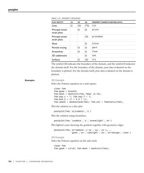
- Page 365 and 366: postplot TABLE 1-31: VALID PROPERTY
- Page 367 and 368: postplot TABLE 1-31: VALID PROPERTY
- Page 369 and 370: postplot TABLE 1-31: VALID PROPERTY
- Page 371 and 372: postplot TABLE 1-31: VALID PROPERTY
- Page 373 and 374: postplot TABLE 1-31: VALID PROPERTY
- Page 375: postplot associated to each point o
- Page 379 and 380: postprincbnd postprincbnd Purpose S
- Page 381 and 382: postsurf postsurf Purpose Shorthand
- Page 383 and 384: pyramid2, pyramid3 Purpose pyramid2
- Page 385 and 386: ect1, rect2 Purpose rect1, rect2 Cr
- Page 387 and 388: evolve Purpose revolve Revolve a 2D
- Page 389 and 390: otate e1 = ellip2(0,0,1,3); e2 = ro
- Page 391 and 392: sharg_2_5 Purpose sharg_2_5 Create
- Page 393 and 394: shcurl Purpose shcurl Create a vect
- Page 395 and 396: shdisc Purpose shdisc Create a disc
- Page 397 and 398: shgp Purpose shgp Create a Gauss-po
- Page 399 and 400: shlag Purpose shlag Create a Lagran
- Page 401 and 402: solid0, solid1, solid2, solid3 The
- Page 403 and 404: sphere3, sphere2 the evaluation con
- Page 405 and 406: square1, square2 Purpose square1, s
- Page 407 and 408: tangent Purpose tangent Create a ta
- Page 409 and 410: tetrahedron2, tetrahedron3 Purpose
- Page 411 and 412: torus2, torus3 TABLE 1-49: TORUS OB
- Page 413 and 414: xmeshinfo is requested for. The pro
- Page 415 and 416: xmeshinfo TABLE 1-52: NODES STRUCT
- Page 417 and 418: xmeshinfo dofs.coords(:,30) % alter
- Page 419 and 420: 2 Diagnostics This chapter contains
- Page 421 and 422: TABLE 2-2: GEOMETRY MODELING ERROR
- Page 423 and 424: 6000-6999 Assembly and Extended Mes
- Page 425 and 426: TABLE 2-4: ASSEMBLY AND EXTENDED ME
- Page 427 and 428:
TABLE 2-5: SOLVER ERROR MESSAGES ER
- Page 429 and 430:
9000-9999 General Errors TABLE 2-6:
- Page 431 and 432:
Solver Error Messages These error m
- Page 433 and 434:
TABLE 2-7: SOLVER ERROR MESSAGES IN
- Page 435 and 436:
3 The COMSOL Multiphysics Files Thi
- Page 437 and 438:
2 m1 ######## Types 1 # number of t
- Page 439 and 440:
To load and save COMSOL Multiphysic
- Page 441 and 442:
Attribute Attribute Supported Versi
- Page 443 and 444:
BezierMfd BezierMfd Supported Versi
- Page 445 and 446:
BezierTri BezierTri Supported Versi
- Page 447 and 448:
BSplineMfd BSplineMfd Supported Ver
- Page 449 and 450:
BSplineSurf BSplineSurf Supported V
- Page 451 and 452:
Ellipse 0 # reverse 2 0 # major axi
- Page 453 and 454:
Geom1 Geom1 Supported Versions 1 Su
- Page 455 and 456:
Geom2 0 0 1 1 2.2999999999999998 1
- Page 457 and 458:
GeomFile GeomFile Supported Version
- Page 459 and 460:
Mesh Mesh Supported Versions 1 Subt
- Page 461 and 462:
MeshCurve MeshCurve Supported Versi
- Page 463 and 464:
Plane Plane Supported Versions 1 Su
- Page 465 and 466:
Serializable Serializable Supported
- Page 467 and 468:
Transform Transform Supported Versi
- Page 469 and 470:
VectorInt Supported Versions Vector
- Page 471 and 472:
Examples To illustrate the use of t
- Page 473 and 474:
410 506 409 528 762 760 831 859 525
- Page 475 and 476:
7 ... 5 5 5 224 # number of up/down
- Page 477 and 478:
# Faces # up down mfd tol 0 0 1 NAN
- Page 479 and 480:
INDEX 1D geometry object 196 3D mes
- Page 481 and 482:
flmesh2spline 186 flngdof 188, 191
- Page 483 and 484:
second fundamental matrices 226 ser