Cost-Based Optimization of Integration Flows - Datenbanken ...

6.4 Optimization Techniques
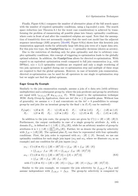
Finally, Figure 6.9(c) compares the number of alternative plans of the full search space
with the number of required optimality conditions, using a log-scaled y-axis. The search
space reduction (see Theorem 6.1 for the worst case consideration) is achieved by transforming
the problem of enumerating all possible plans into binary optimality conditions,
where costs in front of and after the considered subplan are equal. Note that the assumption
of transitivity does not necessarily require that the used cost model has the adjacent
sequence interchange (ASI) property [Moe09]. Figure 6.9(a) shows how this heuristic join
enumeration approach works for arbitrarily large left-deep join trees of n input data sets.
For this join tree type, the PlanOptTree has n − 1 optimality decisions (shown as arrows).
Due to the restriction of checking only for plan optimality and due to arbitrary complex
optimality conditions, this concept of triggering re-optimization leads to the globally
optimal solution. In addition, the PlanOptTree allows for directed re-optimization. With
regard to an equivalent optimization result compared to full join enumeration (e.g., with
DPSize), n(n + 1)/2 optimality conditions are required and only a single reordering of
two join operators is applied during one re-optimization step and multiple of these steps
are required to find the global optimum. However, in case of heuristic join enumeration,
directed re-optimization can be used for all operators in one single re-optimization step
but we might not find the global optimum.
Eager Group-By Example
Similarly to the join enumeration example, assume a join of n data sets (with arbitrary
multiplicities) and a subsequent group-by, where the join predicate and group-by attributes
are equal with γ F (X);A1 (R ⋊⋉ R.A1 =S.A 1
S). With regard to the optimization technique
WD6: Early Group-by Application, there are 4n! (for n ≥ 2) possible plans. Without loss
of generality, we assume n = 2 and concentrate on the 4n! = 8 possibilities to arrange
group-by and join (for an invariant group-by the final γ in P c -P f can be omitted):
P a (opt) : γ(R ⋊⋉ S) P c : γ((γR) ⋊⋉ S) P e : γ(R ⋊⋉ (γS)) P g : (γR) ⋊⋉ (γS)
P b : γ(S ⋊⋉ R) P d : γ(S ⋊⋉ (γR)) P f : γ((γS) ⋊⋉ R) P h : (γS) ⋊⋉ (γR).
In addition to the join costs, the group-by costs are given by C(γ) = |R| + |R| · |R|/2.
Furthermore, the output cardinality in case of a single group-by attribute A i , with a
domain D Ai , is defined as 1 ≤ |γR| ≤ |D Ai (R)|, while for an arbitrary number of group-by
attributes it is 1 ≤ |γR| ≤ ∏ |A|
i=1 |D A i
(R)|. Further, let us denote the group-by selectivity
with f γR = |γR|/|R|. The optimal plan P a can then be represented with four optimality
conditions. First, the join order is expressed with oc 1 : |R| ≤ |S|. Second, we use one
optimality condition for each single join input (oc 2 and oc 3 , where we illustrate oc 2 as an
example) and one condition for all join inputs (oc 4 ):
oc 2 : C(γ(R ⋊⋉ S)) ≤ ( |R| + |R| 2 /2 ) + (f γR · |R| + f γR · |R| · |S|)
+ ( f (γR),S · f γR · |R| · |S| + (f (γR),S · f γR · |R| · |S|) 2 /2 )
oc 4 : C(γ(R ⋊⋉ S)) ≤ ( |R| + |R| 2 /2 ) + ( |S| + |S| 2 /2 )
+ (f γR · |R| + f γR · |R| · f γS · |S|)
with C(γ(R ⋊⋉ S)) = (|R| + |R| · |S|) + ( f R,S · |R| · |S| + (f R,S · |R| · |S|) 2 /2 ) .
(6.6)
Similar to the join example, we compute the join selectivity by f (γR),S θ f R,S and
assume independence with f (γR),S = f R,S . The group-by selectivity is computed by
183