Cost-Based Optimization of Integration Flows - Datenbanken ...

3 Fundamentals of Optimizing Integration Flows
of C(⋊⋉) = |R| + |R| · |S|, the group-by costs are given by C(γ) = |R| + |R| · |R|/2.
Furthermore, the output cardinality in case of a single group-by attribute A i is defined
as 1 ≤ |γR| ≤ |D Ai (R)|, while for an arbitrary number of group-by attributes it is
1 ≤ |γR| ≤ ∏ |A|
i=1 |D A i
(R)|, where D Ai denotes the domain of an attribute A i . Further, we
denote the group-by selectivity with f γR = |γR|/|R|. Then, the plan P a is optimal if the
following four optimality conditions hold. First, the commutative join order is expressed
with |R| ≤ |S|. Second, there is one optimality condition for each single join input (in
order to determine if pre-aggregation is advantageous):
C(γ(R ⋊⋉ S)) ≤ ( |R| + |R| 2 /2 ) + (f γR · |R| + f γR · |R| · |S|)
+ ( f (γR),S · f γR · |R| · |S| + (f (γR),S · f γR · |R| · |S|) 2 /2 )
with C(γ(R ⋊⋉ S)) = (|R| + |R| · |S|) + ( f R,S · |R| · |S| + (f R,S · |R| · |S|) 2 /2 ) ,
(3.24)
C(γ(R ⋊⋉ S)) ≤ ( |S| + |S| 2 /2 ) +(|R| + |R| · f γS · |S|)+ ( |R| + (f R,(γS) · f γS · |R| · |S|) 2 /2 ) ,
(3.25)
and one condition for all join inputs:
C(γ(R ⋊⋉ S)) ≤ ( |R| + |R| 2 /2 ) + ( |S| + |S| 2 /2 ) + (f γR · |R| + f γR · |R| · f γS · |S|). (3.26)
These conditions are necessary due to the characteristic of missing knowledge about data
properties. For example, we do not know the multiplicities of join inputs that can be
exploited for defining simpler optimality conditions in advance. The algorithm for realizing
this technique is invoked for each Groupby operator. Then, we check by the use of the
dependency graph if this operator can be reordered with predecessor Join operators, where
for each join there are four optimality conditions. As a result, this algorithm exhibits a
linear time complexity of O(m). We use an example to illustrate this concept.
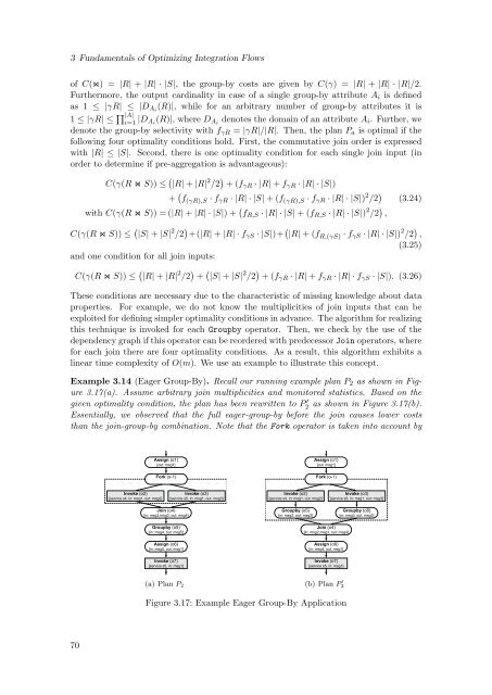
Example 3.14 (Eager Group-By). Recall our running example plan P 2 as shown in Figure
3.17(a). Assume arbitrary join multiplicities and monitored statistics. Based on the
given optimality condition, the plan has been rewritten to P 2 ′ as shown in Figure 3.17(b).
Essentially, we observed that the full eager-group-by before the join causes lower costs
than the join-group-by combination. Note that the Fork operator is taken into account by
Assign (o1)
[out: msg1]
Fork (o-1)
Assign (o1)
[out: msg1]
Fork (o-1)
Invoke (o2)
[service s4, in: msg1, out: msg2]
Invoke (o3)
[service s5, in: msg1, out: msg3]
Invoke (o2)
[service s4, in: msg1, out: msg2]
Invoke (o3)
[service s5, in: msg1, out: msg3]
Join (o4)
[in: msg2,msg3, out: msg4]
Groupby (o5)
[in: msg2, out: msg2]
Groupby (o8)
[in: msg3, out: msg3]
Groupby (o5)
[in: msg4, out: msg5]
Assign (o6)
[in: msg5, out: msg1]
Invoke (o7)
[service s5, in: msg1]
Join (o4)
[in: msg2,msg3, out: msg4]
Assign (o6)
[in: msg4, out: msg1]
Invoke (o7)
[service s5, in: msg1]
(a) Plan P 2
(b) Plan P ′ 2
Figure 3.17: Example Eager Group-By Application
70