Cost-Based Optimization of Integration Flows - Datenbanken ...

3.3 Periodical Re-Optimization
Join (o14)
[in: msg1,msg9, out: msg13]
Join (o15)
[in: msg13,msg12, out: msg14]
Join (o16)
[in: msg14,msg4, out: msg15]
Join (o17)
[in: msg15,msg7, out: msg16]
Assign (o18)
[in: msg16, out: msg17]
Invoke (o19)
[service s6, in: msg17]
INNER
INNER
INNER
INNER
Join (o14)
[in: msg1,msg9, out: msg13]
Join (o15)
[in: msg13,msg12, out: msg14]
Join (o16)
[in: msg14,msg4, out: msg15]
Invoke (o19)
[service s6, in: msg15]
Join (o17)
[in: msg15,msg7, out: msg16]
INNER
INNER
INNER
INNER
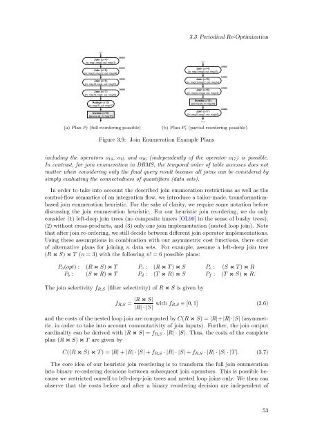
(a) Plan P 7 (full reordering possible)
(b) Plan P ′ 7 (partial reordering possible)
Figure 3.9: Join Enumeration Example Plans
including the operators o 14 , o 15 and o 16 (independently of the operator o 17 ) is possible.
In contrast, for join enumeration in DBMS, the temporal order of table accesses does not
matter when considering only the final query result because all joins can be considered by
simply evaluating the connectedness of quantifiers (data sets).
In order to take into account the described join enumeration restrictions as well as the
control-flow semantics of an integration flow, we introduce a tailor-made, transformationbased
join enumeration heuristic. For the sake of clarity, we require some notation before
discussing the join enumeration heuristic. For our heuristic join reordering, we do only
consider (1) left-deep join trees (no composite inners [OL90] in the sense of bushy trees),
(2) without cross-products, and (3) only one join implementation (nested loop join). Note
that after join re-ordering, we still decide between different join operator implementations.
Using these assumptions in combination with our asymmetric cost functions, there exist
n! alternative plans for joining n data sets. For example, assume a left-deep join tree
(R ⋊⋉ S) ⋊⋉ T (n = 3) with the following n! = 6 possible plans:
P a (opt) : (R ⋊⋉ S) ⋊⋉ T P c : (R ⋊⋉ T ) ⋊⋉ S P e : (S ⋊⋉ T ) ⋊⋉ R
P b : (S ⋊⋉ R) ⋊⋉ T P d : (T ⋊⋉ R) ⋊⋉ S P f : (T ⋊⋉ S) ⋊⋉ R.
The join selectivity f R,S (filter selectivity) of R ⋊⋉ S is given by
f R,S =
|R ⋊⋉ S|
|R| · |S| with f R,S ∈ [0, 1] (3.6)
and the costs of the nested loop join are computed by C(R ⋊⋉ S) = |R|+|R|·|S| (asymmetric,
in order to take into account commutativity of join inputs). Further, the join output
cardinality can be derived with |R ⋊⋉ S| = f R,S · |R| · |S|. Thus, the costs of the complete
plan (R ⋊⋉ S) ⋊⋉ T are given by
C((R ⋊⋉ S) ⋊⋉ T ) = |R| + |R| · |S| + f R,S · |R| · |S| + f R,S · |R| · |S| · |T |. (3.7)
The core idea of our heuristic join reordering is to transform the full join enumeration
into binary re-ordering decisions between subsequent join operators. This is possible because
we restricted ourself to left-deep-join trees and nested loop joins only. We then can
observe that the costs before and after a binary reordering decision are independent of
53