Cost-Based Optimization of Integration Flows - Datenbanken ...

3 Fundamentals of Optimizing Integration Flows
Definition 3.4 (Periodic Plan Optimization Problem (P-PPO 3 )). The P-PPO describes
the periodical creation of the optimal plan P at timestamp T k with the period ∆t (optimization
interval). The workload W (P, T k ) is available for a sliding time window of size
∆w. Optimization required an execution time T Opt with T Opt = T k,1 − T k,0 and T k = T k,0 .
When solving the P-PPO at timestamp T k,1 , the result is the optimal plan w.r.t. the
statistics available at timestamp T k,0 .
∆t(P)
∆t(P)
∆w(P)
Workload W(P,Tk)
Topt(P)
∆w(P)
Workload W(P,Tk)
Topt(P)
∆w(P)
Workload W(P,Tk+1)
Topt(P)
Opti
Opti
Opti+1
Tk-1
Tk
Tk+1
time t
Tk-1,0
Tk-1,1
Tk,0 Tk,1 Tk+1,0 Tk+1,1
Figure 3.5: Temporal Aspects of the P-PPO
Figure 3.5 illustrates the temporal aspects of periodical re-optimization in more detail.
We optimize the given plan at timestamp T k with a period of ∆t. During this optimization,
we evaluate costs of a plan by double-metric cost estimation, where only statistics in the
interval of [T k − ∆w, T k ] are taken into account. The parameters optimization interval
∆t and workload sliding time window size ∆w are set individually for each plan P . We
will revisit the influence of these parameters in Subsection 3.3.3. The following example
illustrates this concept of periodical re-optimization and shows how the introduced cost
estimation approach is used in this context.
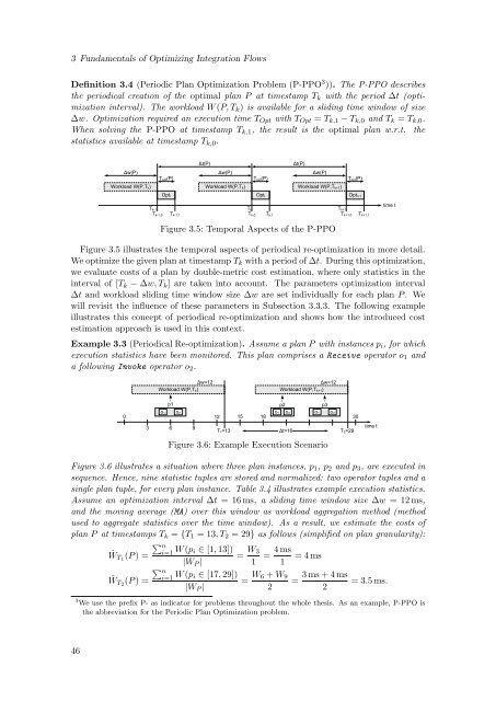
Example 3.3 (Periodical Re-optimization). Assume a plan P with instances p i , for which
execution statistics have been monitored. This plan comprises a Receive operator o 1 and
a following Invoke operator o 2 .
∆w=12
Workload W(P,Tk)
∆w=12
Workload W(P,Tk+1)
p1
p2
p3
o1
o2
0 12 15 18
30
3 6 9
T1=13
∆t=16
T2=29
Figure 3.6: Example Execution Scenario
o1
o2
o1
o2
time t
Figure 3.6 illustrates a situation where three plan instances, p 1 , p 2 and p 3 , are executed in
sequence. Hence, nine statistic tuples are stored and normalized: two operator tuples and a
single plan tuple, for every plan instance. Table 3.4 illustrates example execution statistics.
Assume an optimization interval ∆t = 16 ms, a sliding time window size ∆w = 12 ms,
and the moving average (MA) over this window as workload aggregation method (method
used to aggregate statistics over the time window). As a result, we estimate the costs of
plan P at timestamps T k = {T 1 = 13, T 2 = 29} as follows (simplified on plan granularity):
∑ n
i=1
Ŵ T1 (P ) =
W (p i ∈ [1, 13])
= W 3
|W P |
1 = 4 ms = 4 ms
1
∑ n
i=1
Ŵ T2 (P ) =
W (p i ∈ [17, 29])
|W P |
= W 6 + W 9
2
=
3 ms + 4 ms
2
= 3.5 ms.
3 We use the prefix P- as indicator for problems throughout the whole thesis. As an example, P-PPO is
the abbreviation for the Periodic Plan Optimization problem.
46