Cost-Based Optimization of Integration Flows - Datenbanken ...

3 Fundamentals of Optimizing Integration Flows
1,000
1,000
W
W
600,000
V
600,000
T
T
V
R
S
R
S
(a) Plan P (before reordering)
(b) Plan P ′ (after reordering)
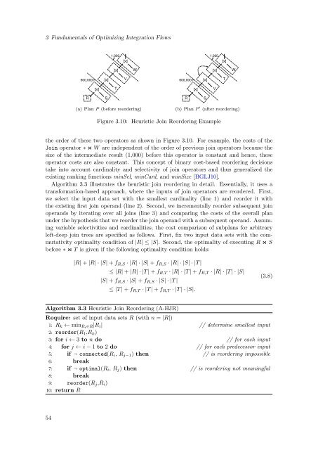
Figure 3.10: Heuristic Join Reordering Example
the order of these two operators as shown in Figure 3.10. For example, the costs of the
Join operator ∗ ⋊⋉ W are independent of the order of previous join operators because the
size of the intermediate result (1,000) before this operator is constant and hence, these
operator costs are also constant. This concept of binary cost-based reordering decisions
take into account cardinality and selectivity of join operators and thus generalized the
existing ranking functions minSel, minCard, and minSize [BGLJ10].
Algorithm 3.3 illustrates the heuristic join reordering in detail. Essentially, it uses a
transformation-based approach, where the inputs of join operators are reordered. First,
we select the input data set with the smallest cardinality (line 1) and reorder it with
the existing first join operand (line 2). Second, we incrementally reorder subsequent join
operands by iterating over all joins (line 3) and comparing the costs of the overall plan
under the hypothesis that we reorder the join operand with a subsequent operand. Assuming
variable selectivities and cardinalities, the cost comparison of subplans for arbitrary
left-deep join trees are specified as follows. First, fix two input data sets with the commutativity
optimality condition of |R| ≤ |S|. Second, the optimality of executing R ⋊⋉ S
before ∗ ⋊⋉ T is given if the following optimality condition holds:
|R| + |R| · |S| + f R,S · |R| · |S| + f R,S · |R| · |S| · |T |
≤ |R| + |R| · |T | + f R,T · |R| · |T | + f R,T · |R| · |T | · |S|
|S| + f R,S · |S| + f R,S · |S| · |T |
≤ |T | + f R,T · |T | + f R,T · |T | · |S|.
(3.8)
Algorithm 3.3 Heuristic Join Reordering (A-HJR)
Require: set of input data sets R (with n = |R|)
1: R k ← min Ri ∈R|R i | // determine smallest input
2: reorder(R 1 ,R k )
3: for i ← 3 to n do // for each input
4: for j ← i − 1 to 2 do // for each predecessor input
5: if ¬ connected(R i , R j−1 ) then // is reordering impossible
6: break
7: if ¬ optimal(R i , R j ) then // is reordering not meaningful
8: break
9: reorder(R j ,R i )
10: return R
54