Cost-Based Optimization of Integration Flows - Datenbanken ...

3 Fundamentals of Optimizing Integration Flows
In order to achieve control-flow awareness, we additionally need to take into account
the path probabilities of (possibly hierarchically structured) Switch operators in the form
of probabilities P (o i ) that an operator is executed. As a result, the costs of a sequence of
Selection operators are determined by
C(P ) =
=
m∑
(P (o i ) · |ds in (o i )|)
i=1
⎛
⎞
m∑ ∏i−1
(
⎝ P (oj ) · f oj + (1 − P (o j )) ) · |ds in (o 1 )| ⎠ ,
i=1 j=1
(3.23)
where (P (o i ) · f oi + (1 − P (o i ))) denotes the effective operator selectivity. The order of
Selection operators is still optimal if f oi ≤ f oi+1 holds for all selective operators due to the
conditional operator execution with P (o i ). However, the effective operator selectivity must
be taken into account when evaluating following operators. If a Switch operator contains
multiple Selection operators (in different paths), we reorder only the complete Switch
operator according to the total effective operator selectivity P (o i ) · f oi + P (o j ) · f oj . The
actual rewriting algorithm works as follows. First, we determine the selectivities of each
individual operator. Second, we reorder the operators according to the given optimality
condition. Third, we evaluate if the increased costs of additional non-selective operators
(such as the Switch operator) are amortized by applying the selective operator earlier.
While the normal selection reordering exhibits a time complexity of O(m log m) due to
the simple sorting according to the selectivities, the control-flow aware selection reordering
exhibits a time complexity of O(m 2 ) = O(m 2 + m log m) because after sorting, for each
operator, we additionally evaluate all subsequent operators. In the following, we use an
example to illustrate the importance of this control-flow aware rewriting.
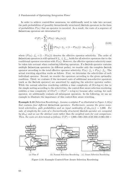
Example 3.13 (Selection Reordering). Assume a subplan P as illustrated in Figure 3.16(a)
that contains four different Selection operators. Furthermore, assume the given monitored
selectivities, path probabilities and an input cardinality of |ds in (o 1 )| = 1,000. For
sake of simplicity the costs of a (hierarchically structured) Switch operator are computed
by |ds in | and we use the abstract costs rather than the weighted costs for cost comparison.
Then, the costs are determined as follows: C(P ) = 1,000+500+350+0.05·350+0.965·350 =
[P(A)=0.9]
f=0.5
Selection (o1)
[in: msg1, out: msg2]
f=0.7
Selection (o2)
[in: msg2, out: msg3]
Switch (o3)
[in: msg3]
f=0.4
Selection (o8)
[in: msg4, out: msg5]
[P(B)=0.1]
Switch (o5)
[in: msg3] [P(D)=0.5]
f=0.3
Selection (o7)
[in: msg3, out: msg4]
[P(A)=0.9]
Switch (o3)
[in: msg3]
f=0.4
Selection (o8)
[in: msg4, out: msg5]
f=0.5
Selection (o1)
[in: msg5, out: msg2]
f=0.7
Selection (o2)
[in: msg2, out: msg3]
[P(B)=0.1]
Switch (o5)
[in: msg3] [P(D)=0.5]
f=0.3
Selection (o7)
[in: msg3, out: msg4]
[P(A)=0.9]
f=0.4
Selection (o8)
[in: msg4, out: msg5]
f=0.5
Selection (o1)
[in: msg5, out: msg2]
f=0.7
Selection (o2)
[in: msg2, out: msg3]
Switch (o3)
[in: msg3]
[P(B)=0.1]
Switch (o5)
[in: msg3] [P(D)=0.5]
f=0.3
Selection (o7)
[in: msg3, out: msg4]
(a) Plan P
(b) Normal Selection Reordering
(c) Aware Selection Reordering
Figure 3.16: Example Control-Flow-Aware Selection Reordering
68