Cost-Based Optimization of Integration Flows - Datenbanken ...

3 Fundamentals of Optimizing Integration Flows
for this example plan, the re-optimization time is dominated by the physical plan compilation
and the waiting time for the next possible exchange of plans. The generation of
physical plans regardless of whether or not a new plan was found has been reasoned by
optimization techniques (such as switch path re-ordering), which directly reorder operators
and thus, they always signal that recompilation is required. Clearly, for periodical
re-optimization, we could use a larger ∆t and thus, would reduce the cumulative total
optimization time. However, in that case, we would use suboptimal plans for a longer
time and hence, we would miss more optimization opportunities.
Furthermore, Figures 3.20(d) and 3.20(f) show the execution time using periodical reoptimization
compared to the non-optimized execution. The different execution times
are caused by the changing workload characteristics in the sense of different input cardinalities
as well as selectivities of the different operators. When using periodical reoptimization,
the often re-occurring small peaks are caused by the numerous asynchronous
re-optimization steps. Further, a major characteristic of periodical re-optimization is that
after a certain workload shift, there is an adaptation delay until periodical re-optimization
is triggered. During this time, the execution time of the current plan is much longer than
the execution time of the optimal plan. In order to reduce these adaptation delays, a small
∆t is required. However, this would significantly increase the total re-optimization time.
To summarize, over time, significant execution time reductions are yielded by periodical
re-optimization due to the adaptation to changing workload characteristics.
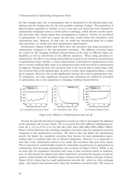
(a) Cumulative Execution Time (b) Cumulative Opt. Time (c) Scenario Elapsed Time
Figure 3.21: Influence of Optimization Interval ∆t
Second, we used the introduced comparison scenario in order to investigate the influence
of the parameter ∆t in more detail. We re-executed this with different optimization periods
∆t ∈ {1 s, 2 s, 3.75 s, 7.5 s, 15 s, 30 s, 60 s, 120 s, 240 s, 480 s, 960 s 1800 s, 3600 s, 7200 s}.
Figure 3.21(a) illustrates the resulting cumulative execution time for optimized execution
compared to the unoptimized execution. We observe that the higher the optimization
period, the higher the cumulative execution time because we miss optimization opportunities
after a workload shift due to deferred adaptation. However, it is important to
note that if the optimization period is too small, the execution time gets worse again.
This is reasoned by small benefits reached by immediate asynchronous re-optimization in
combination with increasing optimization costs as shown in Figure 3.21(b). While, so far
we used only the cumulative execution time (sum of plan execution times) as indicator,
now, we also discuss the elapsed time (time required for executing the sequence of plan instances,
which includes the workflow engine overhead and time during exchange of plans).
Figure 3.21(c) shows that for small optimization intervals ∆t—where we often exchange
plans—the elapsed time increase faster than the cumulative execution time. The reason is
76