Cost-Based Optimization of Integration Flows - Datenbanken ...

6.4 Optimization Techniques
For arbitrary cardinalities, the optimality conditions (Figures 6.11(a) and 6.11(b)) are
oc 1 : |R| ≥ |S| and
oc 2 : |R| + |S| ·
|R ∪ S|
2
≤ |R| + |S| + |R| · log 2 |R| + |S| · log 2 |S|.
(6.8)
After simplification of oc 2 , we obtain
(
oc ′ 2 : |R ∪ S| ≤ 2 1 + |R| · log )
2|R|
+ log
|S|
2 |S| . (6.9)
Figure 6.11(b) illustrates the resulting PlanOptTree, where we monitor the input and
output cardinalities |R|, |S|, |R ∪ S| and we only have to check the two fairly simple
optimality conditions oc 1 and oc ′ 2 , respectively. A similar concept is also used for example,
when deciding on nested-loop or sort-merge joins.
6.4.2 Cost-Based Vectorization
The concept of on-demand re-optimization can also seamlessly be applied to the controlflow-oriented
technique cost-based plan vectorization that has been presented in Chapter
4. For this technique, the created PlanOptTree depends on the used algorithm and
optimization objective. In this subsection, we illustrate the on-demand re-optimization
for the, already discussed, constrained optimization objective of
⎛ ⎞
φ c = min
m
l k | ∀i ∈ [1, k] : ∑ bi
⎝ W (o j ) ⎠ ≤ W (o max ) + λ, (6.10)
k=1
and the typically used heuristic computation approach (A-CPV), whose core idea is to
merge buckets in a first-fit (next-fit) manner.
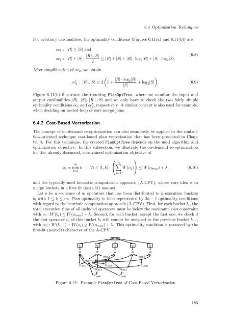
Let o be a sequence of m operators that has been distributed to k execution buckets
b i with 1 ≤ k ≤ m. Plan optimality is then represented by 2k − 1 optimality conditions
with regard to the heuristic computation approach (A-CPV). First, for each bucket b i , the
total execution time of all included operators must be below the maximum cost constraint
with oc : W (b i ) ≤ W (o max ) + λ. Second, for each bucket, except the first one, we check if
the first operator o i of this bucket b i still cannot be assigned to the previous bucket b i−1
with oc i : W (b i−1 ) + W (o i ) ≥ W (o max ) + λ. This optimality condition is reasoned by the
first-fit (next-fit) character of the A-CPV.
j=1
o 1 o 2 o 3 o 4 o 5
W
max + λ
W
W(b 2)
W W W
W(b 3)
≤ (oc1)
≥ (oc2)
W(b 1+) W(b 2+)
≥ (oc3)
< (oc4) < (oc5)
Figure 6.12: Example PlanOptTree of Cost-Based Vectorization
185