Cost-Based Optimization of Integration Flows - Datenbanken ...

3 Fundamentals of Optimizing Integration Flows
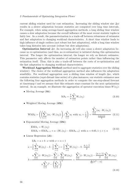
current sliding window used for cost estimation. Increasing the sliding window size ∆w
results in a slower adaptation because statistics are computed over long time intervals.
For example, when using average-based aggregation methods, a long sliding time window
causes a slow adaptation because the overall influence of the most recent statistic tuples is
fairly low. As a result, the parameterization is a trade-off between robustness of estimates
and fast adaptation to changing workload characteristics. A short time window leads to
high influence of single outliers (not robust but fast adaptation), while a long time window
takes long histories into account (robust but slow adaptation).
Optimization Interval ∆t: An increasing ∆t will also cause a slower adaptation because
no re-optimization (and thus, no re-estimation) is initiated during this optimization
interval. The longer the optimization interval, the longer we rely on historic estimates.
This parameter only affects the number of estimation points rather than influencing the
estimation itself. Thus, this is also a trade-off between the costs of re-optimization and
the fast adaptation to changing workload characteristics.
Workload Aggregation Method (method used to aggregate statistics over the sliding
window): The choice of the workload aggregation method also influences the adaptation
sensibility. For workload aggregation over a sliding time window of length ∆w, which
contains statistics (equi-distant time series) of n plan instances, our statistic estimator uses
the following four aggregation methods in order to compute the one-step-ahead forecast
at timestamp t and we assume that this estimate stays constant for the next optimization
interval. As an example, we illustrate the aggregation of operator execution times W (o j ):
• Moving Average (MA):
• Weighted Moving Average (WMA):
(( n∑
WMA t = (w i · W i (o j ))
i=1
• Exponential Moving Average (EMA):
MA t = 1 n
)
/
n∑
W i (o j ) (3.10)
i=1
)
n∑
w i with w i = i =
2
i=1
n∑
(w i · W i (o j ))
i=1
n·(n+1)
4
(3.11)
EMA 1 = W i (o j )
EMA t = EMA t−1 + α · (W i (o j ) − EMA t−1 ) with α = 0.05, 1 ≤ i ≤ n
(3.12)
• Linear Regression (LR):
LR t = a + b · x with x = n + 1
a = 1 n∑
W i (o j ) − b · 1 n∑
i = 1 n∑
W i (o j ) − b · n + 1
n
n n
2
i=1
i=1 i=1
n∑
n∑ n∑
n∑
n (i · W i (o j )) − i · W i (o j ) (i · W i (o j )) −
b =
i=1
n
i=1
i=1
(
n∑ n∑
) 2
=
i 2 − i
i=1
i=1
i=1
(n + 1)
2
1
12 (n3 − n)
n∑
W i (o j )
i=1
.
(3.13)
56